Chap.II Machine Learning 机器学习

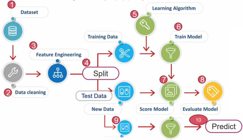
https://yourfreetemplates.com/free-machine-learning-diagram/

Part 3. Learning Algorithm 演算法

本篇会着重在先前提过的监督式学习上。
依据资料类型不同，监督式学习又分以下两种：

Classification 分类

资料集以＂有限的类别＂分布，对於其做归类，即分类。

Regresssion 回归

资料集以＂连续的方式分布＂，对於其以线性方式描述，即回归。

3-1. Weak Learning 弱学习器

概念是由 Michael Kearns 提出，指一个训练模型结果只比随机分类好一点的演算法，称弱学习器。
反之，强学习器则是指经演算法训练後，模型预测结果非常接近真实情况。

以下会以 breast_cancer（Classification）资料来介绍常见的弱学习器：

import pandas as pd
from sklearn import datasets

ds = datasets.load_breast_cancer()
X=pd.DataFrame(ds.data, columns=ds.feature_names)
y=pd.DataFrame(ds.target, columns=['Cancer'])

from sklearn.model_selection import train_test_split
X_train, X_test, y_train, y_test = train_test_split(X, y, test_size = 0.3)

from sklearn.preprocessing import StandardScaler
sc = StandardScaler()
X_train_std = sc.fit_transform(X_train)
X_test_std = sc.fit_transform(X_test)

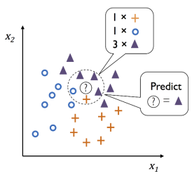
A. K-Nearest Neighbors (KNN) 最近距离法

寻找距离预测值最近的 N 个样本点，以多数决（Majority Voting）决定所属分类。

优点：实现只须两个参数 P & 距离函数。
缺点：无法应用於高维度，且不适用类别（定性）特徵（如性别、星期几...等非数字资料）。
常用於推荐商品。

from sklearn.neighbors import KNeighborsClassifier as knn
clf = KNN(n_neighbors = 3)
clf.fit(X_train_std, y_train)

clf.score(X_test, y_test)
>>  0.9707602339181286

超参数：
1. n_neighbors: 预测值须取多少临近点比较。为避免平局常取奇数。
2. metric: 计算距离的公式。

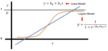
B. Logistic Regresssion 罗吉斯回归

其为线性回归的改良版。（数学原理可参考：推导1、推导2 & 推导3）

优点：Outlier 影响小（上下限 0~1），可线性分割。平滑曲线，变异性小。
缺点：无法应用於高维度、易未拟合，且对於非线性特徵要额外转换。
常用於二分类。

from sklearn.linear_model import LogisticRegression as LR
clf = LR(penalty='l2', C=0.01)
clf.fit(X_train_std, y_train)

clf.score(X_test_std, y_test)

>>  0.9649122807017544

超参数：
1. penalty: 正则化参数。预设 l2。（详细解说）
L1: 将没有用的权重设为0，留下模型认为重要的权重
L2: 削弱所有权重（但仍保留），让所有权重与神经元都处於活动状态。
2. C: 正则化强度的倒数。C 越小，矫正强度越大（使训练分数降低、预测资料变准）。

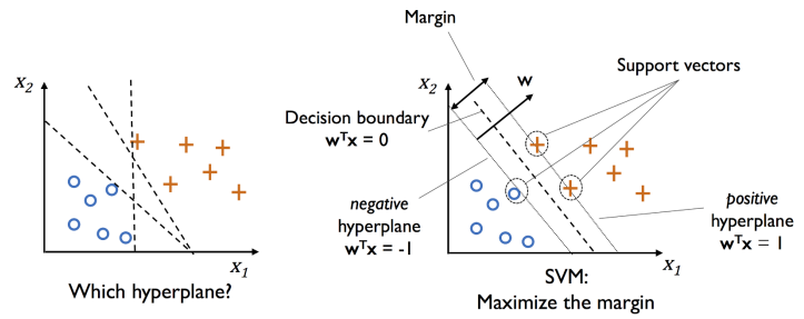
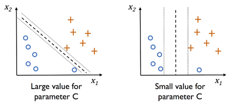
C. Support Vector Machine 支援向量机（SVM）

如图，距离 model（方程序）最近的点，称为 Support Vector 支援向量，
而 positive Hyperplane & negative Hyperplane 彼此间距为 margin。
其根本目的为找到一个 Decision Boundary，使切割的 margin 越大越好。

优点：Outlier 影响小（仅边界影响），且记忆体用量小。高维资料表现好。多样核函数以应对资料。
缺点：样本数大时效能差（须来回优化），成本贵。

from sklearn.svm import SVC
clf = SVC(C=1, probability=True)
clf.fit(X_train_std, y_train)

clf.score(X_test_std, y_test)

>>  0.9649122807017544

可以查看其参照多少支援向量：

len(clf.support_vectors_)

>>  97

超参数：
1. C: 正则化强度的倒数。C 越小，矫正强度越大（使训练分数降低、预测资料变准）。
默认 1（hard margin，尽可能找出完美超平面，下图左）。
若 C=0.01，则模型评分会下降至 0.66。

2. kernel: 同 PCA，有 {‘linear’, ‘poly’, ‘rbf’, ‘sigmoid’, ‘precomputed’} 等分类方式。
若使用 'linear' 分析圆形资料，评分会下降许多
3. probability: True 才能使用 predict_proba 呼叫机率。

PS. 此外，sklearn 有提供三种线性分类写法：

# 1. 较常使用
LinearSVC(C=1, loss='hinge')

# 2. 执行效能较差
SVC(kernal='linear', C=1)

# 3. 适合记忆体有限（训练资料很庞大） or Online Training
SGDClassifier(loss='hinge', alpha=1/(m*C))

D. Decision Tree 决策树

透过 training data 的 fearture 学出一系列的问题，然後来推断其分类。

演算法
A. Sklearn 使用的是 Classification and Regression Tree (CART)
特色为依照数值型特徵切割，且一次切割只分为两个点，但同一特徵可多次切割。
B. Chi-squared Automatic Interaction Detection (CHAID)
所有变数转成不连续的组距（discretecized），切割可大於两个点。
C. 其他还有 ID3、ID4.5、ID5.0、Decision Stump、M5...等。

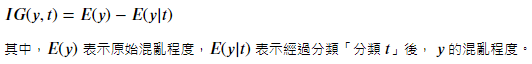
Information gain 信息增益
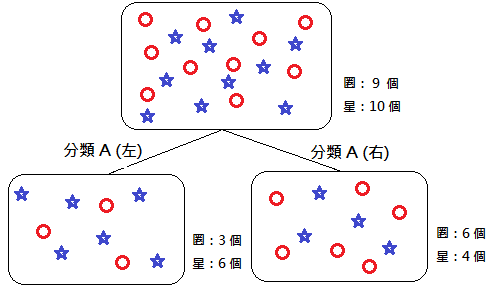
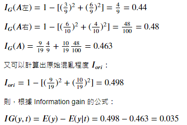
为了能在节点上使用最具意义的特徵来分割，我们会透过信息增益来判断。
信息增益越大，那此「分类」对於决策树来说就越重要，表示它能把数据分的越乾净。
所谓的信息增益，可用以下方式表达：

常见信息增益计算：
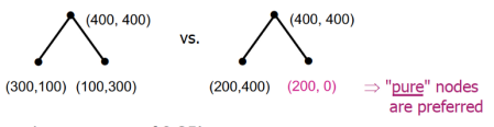
A. Gini Impurity 吉尼不纯度：
计算一「随机样本」被某个「分类 x 」分错的概率。不纯度越低，表示该分类方法越显着有用。

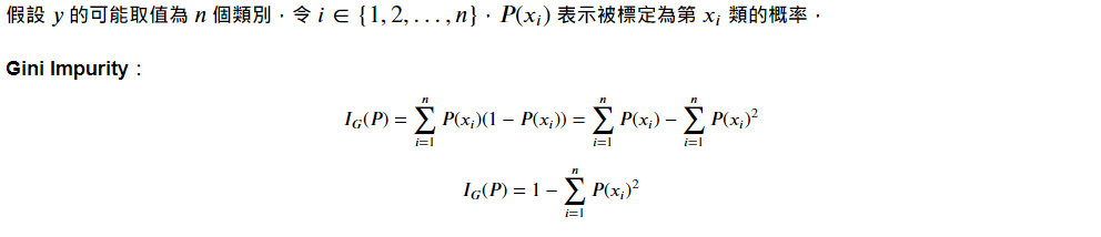
Ex. 假设分类後仅剩下 1 种特徵，则 Ig = 1-(1+0) = 0，为一个不纯度最低的完美分类方法。
（多考虑纯度，故比起 Entropy，分类效果较好）

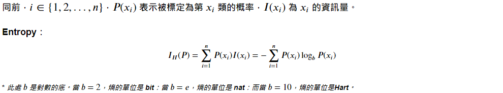
B. Entropy 熵：
类似热力学，但在资讯理论中多了负号。熵高（负少）传输资讯多，熵低（负多）则传输资讯少。

C. Classification Error 分类错误率：
很直观，即分类错误的最小机率。

优点：易於了解与解释（可视觉化）。资料仅须少量前处理（不需常态/标准化）。无复杂计算。
缺点：易过拟合，需搭配特徵选择减少特徵量。不平衡样本（得病/无病）差距太多，会使分割偏向多数样本方，需使用 class balancing 技术（如 SMOTE）矫正。

程序码
*注意!!! 决策树演算不需要标准化/正则化的!!!
它们不关心特徵「值」，只关心特徵「分布」和特徵间的「条件概率」

import pandas as pd
from sklearn import datasets

ds = datasets.load_breast_cancer()
X=pd.DataFrame(ds.data, columns=ds.feature_names)
y=pd.DataFrame(ds.target, columns=['Cancer'])

from sklearn.model_selection import train_test_split
X_train, X_test, y_train, y_test = train_test_split(X, y, test_size = 0.3)

决策树：

from sklearn.tree import DecisionTreeClassifier as DTC
clf = DTC(criterion='gini', max_depth=3, random_state=1)
clf.fit(X_train, y_train)

clf.score(X_test, y_test)

>>  0.9064327485380117

超参数：
1. criterion: 不纯度方法，'gini'（默认） & 'entropy'。
2. max_depth: 树的层数。若 None 则扩展节点至所有叶包含 min_samples_split 样本。默认 None。
3. min_samples_split: 分裂一个内部节点所需的最小样本数。默认 2。
更多参数看 DecisionTreeClassifier或 DecisionTreeRegressor

要让决策树视觉化，需安装以下两个程序：

1. Graphviz (官方网站)
   下载後，进入主机（右键）内容 -> 进阶系统设定 -> 环境变数 -> Path
   并新增＂C:\Users\User.conda\envs\tensorflow-gpu\Lib\site-packages\graphviz\bin＂

2. 使用 pip 安装 pydotplus

pip install pydotplus

正式使用：

# 作图
from pydotplus import graph_from_dot_data
from sklearn.tree import export_graphviz

dot_data = export_graphviz(clf,
                          filled = True,
                          class_names = ds.target_names,
                          feature_names = ds.feature_names,
                          out_file = None)
graph = graph_from_dot_data(dot_data)
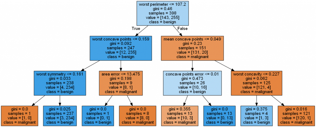
graph.write_png('Pic\Cancer tree.png')

# 显示图片
from IPython.display import Image
Image(filename='Pic\Cancer tree.png', width=1000)

另外，Decision Tree 也可以应用於回归类型的资料，见补充 4.。

结论：

1. KNN: 实现仅需两参数。但高维表现弱。可用於推荐商品。
2. Logistic Regresssion: 以 0~1 分割资料。但高维表现差。可用於二分法演算。
3. SVM: 边界影响小，高维表现好，可分析多种类型（如圆球形）资料。但耗时长成本高。
4. Decision Tree: 可视觉化，资料不需前处理。但易过拟合，且若样本差距过大需矫正。
5. Random Forest: 高维表现好，能平衡资料误差。但记忆体消耗高，且无法针对单一树解释。
   .
   .
   .
   .
   .
   *补充 1.：Gini Impurity
   
   

*补充 2.：Entropy

左右两边的 Etropy 算出来皆为 0.5，但

*补充 3.：客户留存率与流失率

*补充 4.：Decision Tree 回归 Boston

from sklearn.datasets import load_boston
from sklearn.tree import DecisionTreeRegressor as DTR
import pandas as pd

ds = load_boston()
X=pd.DataFrame(ds.data, columns=ds.feature_names)
y=pd.DataFrame(ds.target, columns=['Boston'])

from sklearn.model_selection import train_test_split
X_train, X_test, y_train, y_test = train_test_split(X, y, test_size = 0.3)

clf = DTR(max_depth=2, random_state=1)
clf.fit(X_train, y_train)
clf.score(X_test, y_test)

>>  0.6865210494380858

.
.
.
.
.

Homework Answer：

试着用 sklearn 的资料集 breast_cancer，操作 Featuring Extraction (by PCA)。

# Datasets
from sklearn.datasets import load_breast_cancer
import pandas as pd

ds = load_breast_cancer()

df_X = pd.DataFrame(ds.data, columns=ds.feature_names)
df_y = pd.DataFrame(ds.target, columns=['Cancer or Not'])

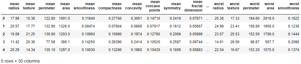
df_X.head()

# define y
df_y['Cancer or Not'].unique()

>>  array([0, 1])

# Split
from sklearn.model_selection import train_test_split

X_train, X_test, y_train, y_test = train_test_split(df_X, df_y, test_size=0.3)
X_train.shape, X_test.shape

>>  ((398, 30), (171, 30))

from sklearn.decomposition import PCA

pca1 = PCA(n_components=2)
X_train_pca = pca1.fit_transform(X_train)
X_test_pca = pca1.transform(X_test)

X_train_pca.shape, X_test_pca.shape

>>  ((398, 2), (171, 2))

# Modeling (by LogisticRegression)
from sklearn.linear_model import LogisticRegression as lr

clf = lr(solver='liblinear')
clf.fit(X_train_pca, y_train)

print(clf.score(X_test_pca, y_test))

>>  0.9298245614035088