前言

昨天我们介绍了FER2013表情资料集，今天要来读取资料与做探索性资料分析。

• Exploratory Data Analysis (EDA)：
  意旨用统计手法分析资料集，取出一些统计值，如样本数、平均数和四分位数。
  也可以用统计图表画出资料的趋势，常见的统计图有直方图、折线图。
  EDA可以帮助我们了解资料的特性，像是qqplot可以看出资料是否接近常态分布。
  常常可以帮我们检验资料是否符合统计分析方法的先前假设(hypothesis)，
  像是变异数分析中(ANOVA)，样本中不同组别的依变项(y)必须符合变异数同质性，
  所做出来的分析结果才会是可信的。

事前准备

你应该要有一个fer2013.csv，与你的python程序码放在同一个资料夹中。

1. 读取套件

import pandas as pd
import numpy as np
import os
import matplotlib.pyplot as plt

2. 读取资料

由於原始资料是长度为2304的字串，每个数字以空格隔开，
所以我们使用np.fromstring把字串转成numpy array，
再用np.reshape转成2维阵列，视为图片的矩阵。

def prepare_data(data):
    """ Prepare data for modeling 
        input: data frame with labels and pixel data
        output: image and label array """

    image_array = np.zeros(shape=(len(data), 48, 48, 1))
    image_label = np.array(list(map(int, data['emotion'])))

    for i, row in enumerate(data.index):
        image = np.fromstring(data.loc[row, 'pixels'], dtype=int, sep=' ')
        image = np.reshape(image, (48, 48, 1))  # 灰阶图的channel数为1
        image_array[i] = image

    return image_array, image_label

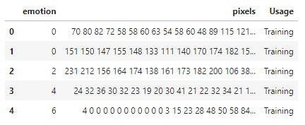
2. 观察资料范例

fer2013.csv只有3个栏位，分别是：

1. emotions: 图片的标签(label)，也是我们的表情类别(y)。
2. pixels: 图片的像素，值域为0 ~ 255。
3. Usage: 该图片用途，分成Training、PublicTest和PrivateTest，前者用来训练，当初比赛最後的冠军是以PrivateTest上的准确率为主，但是在有些论文则会看PublicTest。

3. 切分训练集、公开测试集和私人测试集

有些小夥伴会问：我们不是要做EDA吗？为甚麽要分开资料集呢？
当然！不管是PublicTest还是PrivateTest，都是我们未知的资料，
实务上来说，我们不会获得测试集的数据，更不可能获得测试集的标签。
所以我们要在假装看不见测试集的情况下去理解资料。
通常是把训练集再拆分一些出来成为验证集，以验证集代替测试集去检验模型。
但在这里我们将公开测试集当作验证集、私人测试集当测试集。

X_train, y_train = prepare_data(df_raw[df_raw['Usage'] == 'Training'])
X_val, y_val = prepare_data(df_raw[df_raw['Usage'] == 'PublicTest'])
X_test, y_test = prepare_data(df_raw[df_raw['Usage'] == 'PrivateTest'])

4. 一行指令比较各资料集大小

训练、验证和测试集的比例为8:1:1，非常经典~

df_raw['Usage'].value_counts()  # 8:1:1
# output:
# Training       28709
# PrivateTest     3589
# PublicTest      3589
# Name: Usage, dtype: int64

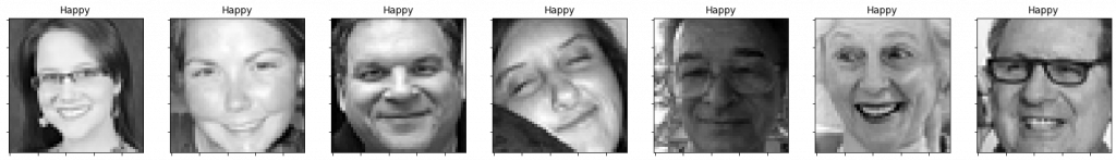
5. 观察每一类的表情图片

历经了重重困难(大约15分钟)，
终於可以观察到活生生的表情图片了！

def plot_one_emotion(data, img_arrays, img_labels, label=0):
    fig, axs = plt.subplots(1, 7, figsize=(25, 12))
    fig.subplots_adjust(hspace=.2, wspace=.2)
    axs = axs.ravel()
    for i in range(7):
        idx = data[data['emotion'] == label].index[i]
        axs[i].imshow(img_arrays[idx][:, :, 0], cmap='gray')
        axs[i].set_title(emotions[img_labels[idx]])
        axs[i].set_xticklabels([])
        axs[i].set_yticklabels([])
        
emotions = {0: 'Angry', 1: 'Disgust', 2: 'Fear',
            3: 'Happy', 4: 'Sad', 5: 'Surprise', 6: 'Neutral'}
for label in emotions.keys():
    plot_one_emotion(df_train, X_train, y_train, label=label)

6. 观察表情分布

def plot_distributions(img_labels_1, img_labels_2, title1='', title2=''):
    df_array1 = pd.DataFrame()
    df_array2 = pd.DataFrame()
    df_array1['emotion'] = img_labels_1
    df_array2['emotion'] = img_labels_2

    fig, axs = plt.subplots(1, 2, figsize=(12, 6), sharey=False)
    x = emotions.values()

    y = df_array1['emotion'].value_counts()
    keys_missed = list(set(emotions.keys()).difference(set(y.keys())))
    for key_missed in keys_missed:
        y[key_missed] = 0
    axs[0].bar(x, y.sort_index(), color='orange')
    axs[0].set_title(title1)
    axs[0].grid()

    y = df_array2['emotion'].value_counts()
    keys_missed = list(set(emotions.keys()).difference(set(y.keys())))
    for key_missed in keys_missed:
        y[key_missed] = 0
    axs[1].bar(x, y.sort_index())
    axs[1].set_title(title2)
    axs[1].grid()

    plt.show()
    
plot_distributions(
    y_train, y_val, title1='train labels', title2='val labels')

资料不平衡的问题苦恼着各个资料科学家，
今天我们发现disgust类别特别少，happy类别特别多。
可能是因为人类是一个友善的族群，
所以当时在蒐集照片时大多是笑脸吧！