机器学习可以分成监督式学习与非监督式学习，这部分我们在第四天有稍微提到过，这边就不多做说明了，今天我们将介绍这两类的问题分别适合用什麽模型来做处理。

一、监督式学习

分类问题

1.罗吉斯回归(Logistic Regression)：

罗吉斯回归是一种分类演算法，其原理为找到一条线将资料尽可能的区隔出来，可以处理二元分类的问题。

• 优点：可解释力强；训练速度快；可获得A类跟B类的机率。
• 缺点：处理非线性数据时较麻烦，需对特徵做更多的处理。

使用鸢尾花资料集(内建)实作

from sklearn import datasets
import pandas as pd
import numpy as np
import matplotlib.pyplot as plt
import seaborn as sns
from sklearn.model_selection import train_test_split
from sklearn.preprocessing import StandardScaler
from sklearn.linear_model import LogisticRegression
from sklearn.metrics import mean_squared_error, accuracy_score
#载入资料集
iris = datasets.load_iris()
#资料整理
x = pd.DataFrame(iris['data'], columns=iris['feature_names'])
y = pd.DataFrame(iris['target'], columns=['target'])
iris_data = pd.concat([x,y], axis=1)#将资料合并
print(iris_data)
#透过两个特徵来进行分类
iris_data = iris_data[['sepal length (cm)','petal length (cm)','target']] 
print(iris_data)
#这边分成两个类别 (山鸢尾、变色鸢尾)
iris_data = iris_data[iris_data['target'].isin([0,1])]
iris_data
X = iris_data[['sepal length (cm)','petal length (cm)']]
y = iris_data[['target']]
#切分训练集以及测试集
X_train, X_test, y_train, y_test = train_test_split(X, y, test_size=0.3, random_state=0)
print('len X_train:',len(X_train),'len X_test:',len(X_test))
#将资料常态分布化，平均值会变为0, 标准差变为1，使离群值影响降低
sc = StandardScaler()
sc.fit(X_train)
X_train_std = sc.transform(X_train)
X_test_std = sc.transform(X_test)
#使用上面整理好切割好的资料做训练
lr = LogisticRegression()
model = lr.fit(X_train_std,y_train['target'].values)
#%%分类预测结果
predict = model.predict(X_test_std)
print("predict label:",predict)
#创建颜色库
markers = ('s', 'x')
colors = ('orange', 'darkblue')
cmap = ListedColormap(colors[:len(np.unique(y))])

#将分类的区块视觉化
x1_min, x1_max = X_train_std[:, 0].min()-1, X_train_std[:, 0].max()+1 # 特徵1最小值与最大值
x2_min, x2_max = X_train_std[:, 1].min()-1, X_train_std[:, 1].max()+1 # 特徵2最小值与最大值
xx1, xx2 = np.meshgrid(np.arange(x1_min, x1_max, 0.01),np.arange(x2_min, x2_max, 0.01)) # 将数据变成m*n矩阵:(m根据前面array长度,n根据後面array长度);0.01为contourf的精度
Z = lr.predict(np.array([xx1.ravel(), xx2.ravel()]).T) #ravel将矩阵拉平成一维
Z = Z.reshape(xx1.shape)

plt.figure(figsize=(12,8))
plt.contourf(xx1, xx2, Z, alpha=0.4, cmap=cmap)
plt.xlim(xx1.min(), xx1.max()) 
plt.ylim(xx2.min(), xx2.max()) #Y轴范围

#画test资料点位置
y_test_n=np.array(y_test.values)#将label data变成跟特徵的类型一样以利後续画图
plt.scatter(X_test_std[:,0], X_test_std[:,1],alpha=0.6,c = y_test_n,edgecolor='black',marker='s')
plt.xlabel('sepal length (cm) [standardized]',size=20)
plt.ylabel('petal width [standardized]',size=20)
plt.show()

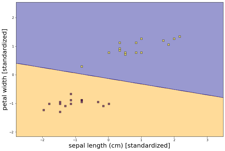
从上图可以看到模型帮助我们找到一条线将资料分成两类。

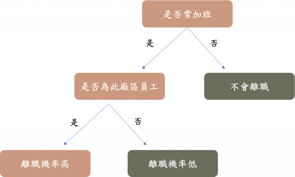
2.决策树(Decision Tree)

透过一系列的是非问题，帮助我们将资料进行切分

• 从训练资料中找出规则，让每一次决策能够使讯息增益最大化
• 讯息增益越大代表切分後的两群资料，群内相似程度越高
• 例如使用员工资料来预测是否离职，若用是否常加班来切分，可以有效分出离职跟非离职的差别，那此特徵就是一个好特徵。(如下图所示)

讯息增益：

用来选特徵的，决策树模型会用特徵切分资料，该选用哪个特徵来切分就是由讯息增益的大小决定的。

clf = tree.DecisionTreeClassifier()
clf = clf.fit(df_X, df_Y)

3.随机森林(Random Forest)

随机森林就是将多个决策树集合而成，为的就是改善决策树容易overfitting的问题，而随机森林也是一种集成学习。

集成 (Ensemble) 就是将多个模型的结果组合在一起，透过投票或是加权的方式得到最终结果，如下图所示：

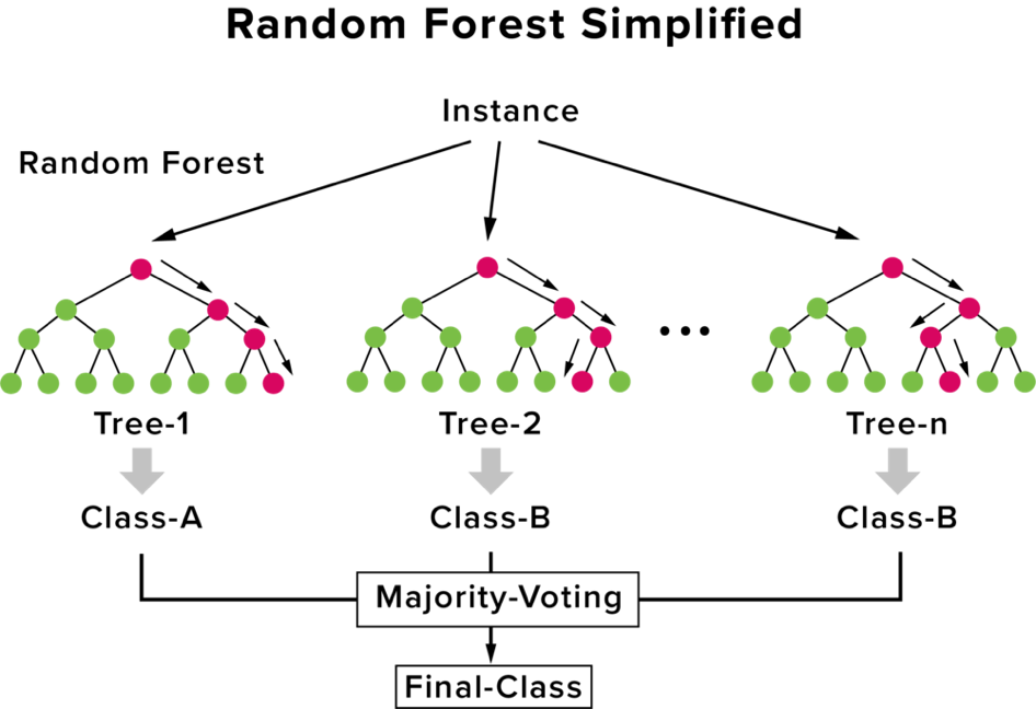
图片来源：机器学习百日马拉松Day43随机森林 (Random Forest) 介绍

from sklearn.ensemble import RandomForestClassifier
rfc=RandomForestClassifier(n_estimators=100)
rfc_model=rfc.fit(df_X,y)
pred_test = rfc_model.predict(data_test)

4.XGboost

XGBoost是boosting算法的其中一种，Boosting算法的概念是将许多弱分类器集成在一起，形成一个强分类器。有兴趣的可以参考原文网址：https://kknews.cc/news/grejk5m.html

from xgboost import XGBClassifier
xgbc=XGBClassifier()
xgbc_model=xgbc.fit(df_X,y)
pred_test = xgbc_model.predict(data_test)

5.支持向量机(Support Vector Classification)

• SVC : Support Vector Classification 支持向量机用於分类问题
• SVR : Support Vector Regression 支持向量机用於回归分析

SVM = SVC()
svc_model = SVM.fit(X_train_std,y_train)

回归问题

1.线性回归模型

线性回归的目的在於找到一条可以拟合数据的线，使预测值与真实值之间的残差越小越好，通常可作为 baseline 模型作为参考点。

使用糖尿病资料集(内建)来实作

# 读取糖尿病资料集
diabetes = datasets.load_diabetes()
x = pd.DataFrame(diabetes['data'],columns=diabetes['feature_names'])
y = pd.DataFrame(diabetes['target'],columns=['target'])
diabetes_data = pd.concat([x,y], axis=1)#将资料合并
diabetes_data
# 取用bmi的特徵
X = np.array(diabetes_data.iloc[:,2:3])
y = np.array(diabetes_data.iloc[:,10:11])
print("Feature shape:", X.shape,"target shape:",y.shape)
#切资料
X_train, X_test, y_train, y_test = train_test_split(X, y, test_size=0.1, random_state=0)
print('len X_train:',len(X_train),'len X_test:',len(X_test))
# 建立一个线性回归模型
reg = LinearRegression()
# 将训练资料丢进去模型训练
reg_model = reg.fit(X_train, y_train)
# 将测试资料丢进模型得到预测结果
y_pred = reg_model.predict(X_test)
# 回归模型的系数与截距
print('coefficients:',reg.coef_)
print('intercept: ',reg.intercept_)
# 预测值与实际值的差距，使用 MSE
print("Mean squared error: %.2f"% mean_squared_error(y_test, y_pred))
# 看模型的准确度
print("R square: %.2f"%r2_score(y_test,y_pred))
#模型效果视觉化
plt.scatter(X_test,y_test,color='black')
plt.plot(X_test, y_pred, color='blue', linewidth=3)
plt.xlabel('bmi',size=20)
plt.ylabel('target',size=20)

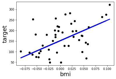
由上图可以看到黑色的点点是我们的预测值

2.随机森林(Random Forest)

# Modeling
rf = RandomForestRegressor(n_estimators = 400, min_samples_leaf=0.12, random_state=123)

#Fitting Random Forest model
rf.fit(X_train, Y_train)

#Predicting using the Random Forest model
Y_pred = rf.predict(X_test)
Y_pred = pd.DataFrame(Y_pred).astype('int')
#Evaluate
print('Mean Absolute Error(MAE):', metrics.mean_absolute_error(Y_test, Y_pred))  
print('Mean Squared Error(MSE):', metrics.mean_squared_error(Y_test, Y_pred))  
print('Root Mean Squared Error(RMSE):', np.sqrt(metrics.mean_squared_error(Y_test, Y_pred)))

3.XGboost

import xgboost
xgb=xgboost.XGBRegressor()
xgb.fit(X_train, Y_train)
xgb_pred = xgb.predict(X_test)

4.支持向量机Support Vector Classification

SVM = SVR()
svr_model = SVM.fit(X_train_std,y_train)

二、非监督式学习

1.K-means(k-平均演算法)

• K-means 目标是使总体群内平方误差最小
• 因爲没有预先的标记，对於 cluster 数量多少才是最佳解，没有标准答案，得靠手动测试观察。
• 当问题不清楚或是资料未有标注的情况下，可以尝试用分群算法帮助了解资料结构，而其中一个方法是运用 K-means 聚类算法帮助分群资料
• 分群算法需要事先定义群数，因此效果评估只能藉由人爲观察。

我们利用内建资料集来实作

import numpy as np
import pandas as pd
from matplotlib import pyplot as plt
from sklearn.datasets import make_blobs  #用於生成聚类资料集
from sklearn.cluster import KMeans
#生成
x, y = make_blobs(n_samples=300, centers=4, cluster_std=3, random_state=0) #cluster_std = The standard deviation of the clusters
df = pd.DataFrame({'x':[x],'y':[y]}) #feature 2 dim ,y=label
plt.scatter(x[:,0], x[:,1],c=y)
x = pd.DataFrame(x,columns=['x1','x2'])
y = pd.DataFrame(y,columns=['y'])

from sklearn.cluster import KMeans
n_clusters=4
kmean = KMeans(n_clusters=n_clusters, random_state=0)
kmean.fit(x)
pred_y = kmean.predict(x)

plt.scatter(x=x.iloc[:,0], y=x.iloc[:,1],c=pred_y)

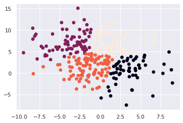
我们设定参数k为四群，而从画出来的图可以看到特徵被有效的分成四群。

三、结论

看到上述的这些模型，是不是觉得头昏脑胀呢？这还只是一小部分而已，之後在这个领域接触的越深，所碰到的资料也会越复杂，甚至还可能需要自己写出一个模型，不过对於初学者来说，能够了解这些模型的原理并知道如何使用它，就可以帮助我们完成一些专案了。