Pima Indians diabetes dataset 考古溯源 & model prediction

Machine learning常用到的一个diabetes 糖尿病资料集，Pima印第安人数据起源於1980年代，目前在机器学习领域还是广为使用，在Kaggle上的运用范例就超过了1700个以上。
我们今天就来探究一下这个资料集。

<资料集来源>：Kaggle download here
from National Institute of Diabetes and Digestive and Kidney Diseases; Includes cost data (donated by Peter Turney)
<资料集说明>来源
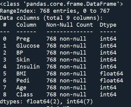
768笔记录。 9个栏位：8 特徵 1 target
This dataset describes the medical records for Pima Indians and whether or not each patient will have an onset of diabetes within five years.
Fields description follow:

1. Preg = Number of times pregnant
2. Glucose = Plasma glucose concentration a 2 hours in an oral glucose tolerance test
3. BP = Diastolic blood pressure (mm Hg)
4. Skin = Triceps skin fold thickness (mm)
5. Insulin = 2-Hour serum insulin (mu U/ml)
6. BMI = Body mass index (weight in kg/(height in m)^2)
7. Pedi = Diabetes pedigree function
8. Age = Age (years)
9. Class = Class variable (1:tested positive for diabetes, 0: tested negative for diabetes)
   < 资料集溯源 >
   我们研读一下原创文献，是如何解释他们的材料方法。
   文献标题：Using the ADAP Learning Algorithm to Forecast the Onset of Diabetes Mellitus
   此研究是由The National Institute of Diabetes Digestive and Kidney Diseases、The Johns Hopkins University School of Medicine共同发表
   1988年原创者文献出处：
   Proc Annu Symp Comput Appl Med Care. 1988 Nov 9 : 261–265.
   8项特徵值之中，比较让人疑惑的是Diabetes pedigree function (糖尿病族谱系数DPF)的定义与计算方法，A function that scores the likelihood of diabetes based on family history.
   我们先把该篇原创论文，摘要的说一遍。
   <研究动机>
   在糖尿病高风险的Pima印第安人族群中，运用ADAP algorithm(一种早期的neural network model)，测试此一方法对於糖尿病发病的预测能力。
   <研究族群>
   Pima印第安人(Phoenix, Arizona)是一批糖尿病高风险发病的族群，该族群居民自1965年起每隔两年都会接受身体检查。如果”口服葡萄糖耐受测试”(oral glucose tolerance test)後的2小时血糖数值，高於200 mg/dl 即视为糖尿病患者。

< 变数选择 > 8项input variables

1. Number of times pregnant 怀孕次数
2. Plasma Glucose Concentration at 2 Hours in an Oral Tolerance Test (GTT) 口服葡萄糖耐受测试後2小时的血糖数据
3. Diastolic Blood pressure 血压(舒张压) mmHg
4. Triceps Skin Fold Thickness (mm) 肱三头肌皮肤厚度
5. 2-Hour Serum Insulin 2小时後血清胰岛素数据
6. Body mass index BMI
7. Diabetes Pedigree Function族谱系数
8. Age (years)年龄

Diabetes Pedigree Function 族谱系数 DPF，此一参数是他们自创的。文中有解释计算方式，有兴趣的请自行参阅。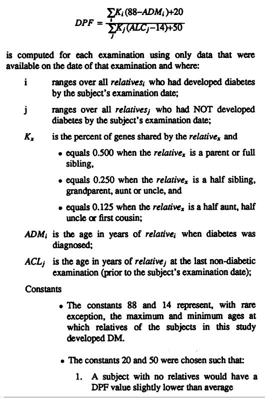

大致意思是：如果家族中得病的人数较多，而这些人发病的年龄比较早，或者亲等关系比较近的，这个DPF数值就会比较高。反之，则DPF数值比较低。
公式大略是以”亲属发病年龄”、”亲等关系比例”…等参数加权计算出来的。

< Case selection >案例选择，必须全部符合以下四项标准：

1. 女性
2. 受测时年龄大於(含)21岁
3. 五年内被诊断出糖尿病者，或者接受GTT口服葡萄糖耐受测试後五年内(或以上)都没有糖尿病者。(这段是我会错意了，文末会说明)
4. 如果受测後一年内诊断出糖尿病者，此记录不采用，剔除研究对象。因为这些数据倾向於比较好预测。
   最後，train组 576例，test组192例，共计768例。
   < ADAP > 作者解释ADAP algorithm作法，我们就不讨论了。

< 资料集表达什麽? >
2014年有篇文章 The Open Diabetes Journal, 2014, 7, 5-13 特讨分析这笔Pima Dataset 得出如下结论：

• Triceps skin fold thickness与PGL(血糖值)有显着的”负相关”
• 2-hr insulin与PGL有显着的”正相关”
• BMI body mass index与PGL有显着的”正相关”
• Diabetes pedigree function与PGL有显着的”正相关”
• Age与PGL有显着的”正相关”
• PGL is independent of number of times pregnant and diastolic blood pressure

我们今天的重点，就是来分析此一资料集，看看能否视觉化，重现上述的相关性，并做modeling、prediction预测
Step1. Read dataset / Explore

''' Step1. Load dataset / explore '''
df = pd.read_csv('pimaDM.csv')
df.isnull().sum()
df.describe()
df.info()
df.head()
df.value_counts()

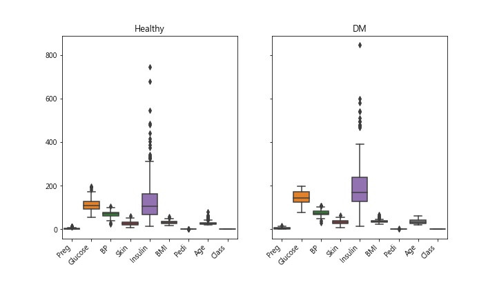
Step 2. data visulalize 画个Box图 观察离散程度
df0 无病组 df1 有病组 把2组画在一起

''' Step 2. data visulalize 
   画个Box图 观察离散程度   '''
# df0 无病组  df1 有病组      
df0 = df[df['Class'] == 0 ]
df1 = df[df['Class'] == 1 ]

# 把2组画在一起
fig,axes = plt.subplots(1,2,sharey=True,figsize=(10,6))

axes[0].set_title('Healthy')
axes[1].set_title('DM')

fig.autofmt_xdate(rotation=45)
sns.boxplot(data=df0,ax=axes[0])
sns.boxplot(data=df1,ax=axes[1])

fig.savefig('DM_orig_box.jpg')

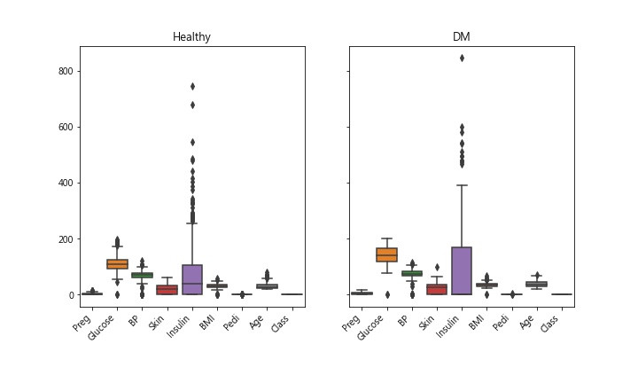
Insulin此特徵数据，离群值似乎很多。算一下统计数据看看

''' Step 3. 统计数据 '''
pd.set_option('display.max_columns',None)  # 显示所有columns
print(df.describe())

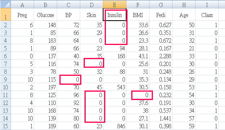
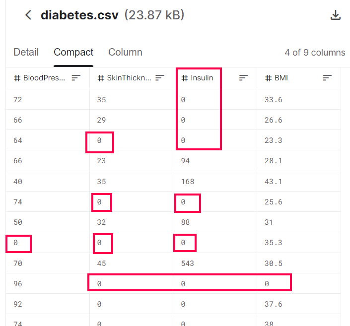
天啊! 出现了很多不合理数据，怎麽说? BP血压是0 ? 皮肤厚度是0 ? 不可能是0，应该是当时没做测量，就随意给个0当数字。

Step 4. 不合理的异常数据处理
血压、皮肤厚度...多项多笔数据=0 明显不合理，将五项特徵 Glucose BP Skin Insulin BMI 数据=0 剔除 ( ps. 原本还包括异常值大於95percentile者，但是资料只剩下三分之一了)

''' Step 4. 不合理的异常数据处理  
    血压、皮肤厚度...多项多笔数据=0 明显不合理
    将五项特徵 Glucose BP Skin Insulin BMI
    数据=0 and >95percentile者剔除
'''
df_Trim = df      # 处理dataframe
# 95 percentile
#Insulin_q95  = df_Trim['Insulin'].quantile(.95)
#print(f'Insulin 95 percentlie: {Insulin_q95}')
#idxNames = df_Trim[ df_Trim['Insulin'] >= Insulin_q95 ].index
#df_Trim = df.drop(idxNames)
# = 0 者
idxNames = df_Trim[ df_Trim['Insulin']<=0 ].index
df_Trim = df_Trim.drop(idxNames)
print(df_Trim.info())
print(df_Trim)
#---以下略---

Step 5. 剩下的资料，再画一次 boxplot
剔除 0 & >95percentile者，剩下 273笔记录 768笔 剩下 35.5% 可用， 如果只剔除 0者，则剩下 392笔记录

< 检视资料 > 用EXCEL检视剩下的资料，虾米!
全部的案例(有病、无病的)“血糖值都小於200”?
糖尿病的定义不是要血糖值大於200吗? 我抓错资料了吗?
再进去Kaggle看看原始资料集。

没错，Kaggle上的资料集和我的是一样的，也都是小於200，Why ?
回头再详细看一看原创文献，Case selection第3项：
Only one examination was selected per subject. 每人只选用一次检验值
That examination was one that revealed a non-diabetic GTT and met one of the following two criteria: 该次检验是在”葡萄糖耐受测试”显示为”非糖尿病”的那次，同时符合以下两标准者：

1. Diabetes was diagnosed within five years of the examination, OR 五年内被诊断出糖尿病，或者
2. A GTT performed five or more years later failed to reveal diabetes mellitus. 5年内(以上)所做的”葡萄糖耐受测试”没有显示出有病者

原来如此，所以，资料集里面的”血糖值”都是正常范围内的，也就是病人”还没被诊断出糖尿病之前”的数据。这就很难理解，这些数据并不是直观的”实验组”、”对照组”的特徵资料，而是”有病者，发病以前的资料”+”没病者的资料”。
所以，该文章作者的方法是：使用”未发病前”的资料去预测以後是否会发病。
说实话，这样的实验设计有点难理解，而且执行上也不容易。
必须要在同一个社区(族群)内，长期追踪同一群人5年以上，收案不易、数据测量也不易齐全。

另外，我们再回头看看上面2014年那篇，好像价值性就没有那麽高了。因为他们在一群正常数据的人(都是未发病前数据)之中发现血糖与其它项特徵值有正(负)相关，但是却没着墨於”预测”。毕竟原创资料集其目的是在於”预测”，而不是看特徵值之”趋势”、”相关”。

Step 6. Prediction
终於，要来使用资料集了。这个资料集去除了不合理的数值後(应该是当时没做测量，就给个0)，剩下392笔可用，只占原本768笔的一半。

经过上面冗长的考古之後，我们就选两种方法来建立模型、预测吧。
LogisticRegression、RandomForest
直接进代码吧

• 准备资料，设定 X ,y
• Build the Model : training
• 评估模型准确度 两种model的accuracy
• 储存模型

''' Step 6. 准备资料，设定 X ,y  '''
from sklearn.model_selection import train_test_split
from sklearn.preprocessing import StandardScaler
 
y = df_Trim['Class']    # y 诊断结果= Class
''' 去除 target栏位，留下特徵栏位-->X '''
X = df_Trim.drop(['Class'], axis = 1)
print(X.shape)
print(X.head(5))   # X is a dataframe
print(y[:5])       # y is a Series

# split dataset
X_train, X_test, y_train, y_test = train_test_split(X, y, 
                                                    test_size=0.2,
                                                    stratify=y,
                                                    random_state=0)

#print(len(X_train),len(X_test))

''' Step 7. Build the Model : training'''

# model logistic regression
from sklearn.linear_model import LogisticRegression

logis = LogisticRegression(solver='lbfgs',max_iter = 400)
logis.fit(X_train, y_train)

# model random forest

from sklearn.ensemble import RandomForestClassifier

fores = RandomForestClassifier()
fores.fit(X_train, y_train)

''' Step 8. 评估模型准确度  两种model的accuracy '''
from sklearn.metrics import accuracy_score

pred_logis = logis.predict(X_test)
pred_fores = fores.predict(X_test)

a1 = accuracy_score(pred_logis, y_test)
a2 = accuracy_score(pred_fores, y_test)
print(f'两种模型的准确率 accuracy: logis: {a1}  fores: {a2}')

''' Step 9. 储存模型  '''
import pickle

mdl_DMlr = 'DMlr.model'
pickle.dump(logis, open(mdl_DMlr, 'wb'))
mdl_DMfs = 'DMfs.model'
pickle.dump(fores, open(mdl_DMfs, 'wb'))
print(' 建模完成 models saved ')

写个py，使用模型预测

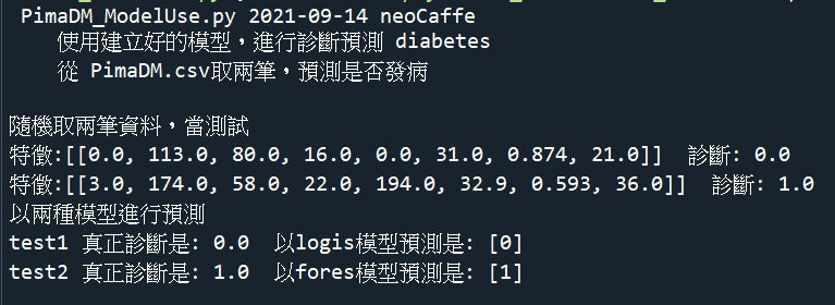
""" PimaDM_ModelUse.py 2021-09-14 neoCaffe
    使用建立好的模型，进行诊断预测 diabetes
    从 PimaDM.csv取两笔，预测是否发病
"""
print(__doc__)

import pandas as pd
import random
import pickle
''' 载入资料集 '''
df = pd.read_csv('pimaDM.csv')
r,c = df.shape
''' 任意取两笔 '''
n = random.randint(0,r)
test1 = list(df.iloc[n].values)
m = random.randint(0,r)
test2 = list(df.iloc[m].values)
# 真正的诊断
Dx1 = test1[-1] 
Dx2 = test2[-1]
# 特徵值
test1 = [test1[:-1]]
test2 = [test2[:-1]]


print('随机取两笔资料，当测试') 
print(f'特徵:{test1}  诊断: {Dx1}')
print(f'特徵:{test2}  诊断: {Dx2}')


''' 以两种模型进行预测  '''
print('以两种模型进行预测''')
mdl_logis = pickle.load(open('DMlr.model', 'rb'))
predict1 = mdl_logis.predict(test1)

mdl_fores = pickle.load(open('DMfs.model', 'rb'))
predict2 = mdl_fores.predict(test2)

print(f'test1 真正诊断是: {Dx1}  以logis模型预测是: {predict1}')
print(f'test2 真正诊断是: {Dx2}  以fores模型预测是: {predict2}')

成果画面

结案收工，以上程序码在GitHub
< source code+csv download GitHub >