资料视觉化 推论统计先 python ANOVA seaborn

在使用seaborn画出炫丽的图片之前，先来做些基本的统计吧。
本文目的：叙述统计、推论统计、视觉直观之组别差异
download here GitHub
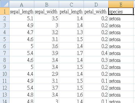
资料集使用的是seaborn提供的iris.csv 长这样，五个栏位(4个特徵、第5个是品种名称)，150笔记录

先使用Excel的oneway ANOVA分析，看看使用这四个特徵是否可以区分出不同的品种(组别)。
Null hypothesis虚无假设：三个品种的特徵平均值，并无差异不同。
P小於0.05 可推翻此null hypothesis
(一)、 EXCEL处理资料
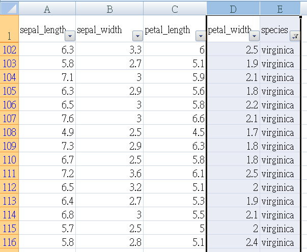
Iris.csv是原始资料模式raw data，无法直接套用 ANOVA ，因为”组别”也在栏位内容中。
我们先”筛选”组别(species)，把四个特值数据复制出来，各自建立一个工作表，第一列写上品种名称。


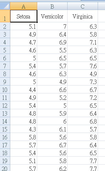
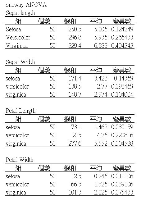
现在，以EXCEL oneway ANOVA (变异数分析)，将四个特徵值各自做一次ANOVA
举例： sepal_length 如下表

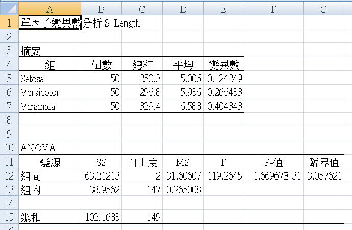
把四个表汇总，如下图。留着等一下验证我们python程序的成果

(二)、代码程序流程：download here GitHub
Step 1. Read csv with dataframe
Step 2. Describe data
Step 3.画个Box图 观察离散程度
Step 4. 画 histogram
Step 5. check if Normal distribution
Step 6. ANOVA test
(三)、解说
Sklearn 、seaborn的范例，总是会po出好几张美美的图，如这张。

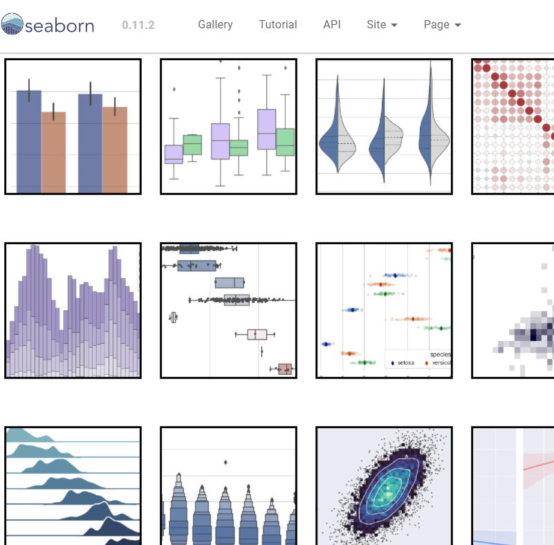
美是美啦，可是，代表啥意思啊?

我们还是先从基本的统计图表来吧。
Descriptive Statistics 先来描述一下资料吧，统计摘要一下iris.csv这个资料集。
可以这样看：平均值 Mean、中位数 Median...

#--- 描述性统计数据
def descrStat(gpdf,fld):
    # 以下码可以用一行 df.describe() 代替之
    SL_min  = gpdf[fld].min()
    SL_max  = gpdf[fld].max()
    SL_mean = gpdf[fld].mean()
    SL_std  = gpdf[fld].std()
    SL_median = gpdf[fld].median()
    SL_var  = gpdf[fld].var()
    SL_q25  = gpdf[fld].quantile(.25)
    SL_q50  = gpdf[fld].quantile(.50)
    SL_q75  = gpdf[fld].quantile(.75) 
    
    print('%s : min %.5f max %.5f mean %.5f std %.5f var %.5f'
          % (fld,SL_min,SL_max,SL_mean, SL_std, SL_var))
    print('median %.5f 25qunatile %.5f 50qunatile %.5f 75qunatile %.5f'
          % (SL_median, SL_q25, SL_q50, SL_q75))

# 只选 setosa这组
df0 = df[df['species']=='setosa']
print('setosa组，统计数据如下：')
print(df0.describe())
#descrStat(df0,'sepal_length')     # 回报统计数据

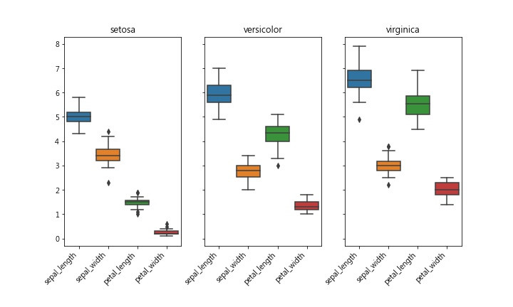
BoxPlot 可看出数据的集中或离散程度，方盒上标75% 下标25%，中间线是平均值。盒子扁的表示大家都”向中靠陇”，反之盒子宽的，彼此”较生疏”…

''' Step 3. 画个Box图 观察离散程度 min mean max percentile '''
import seaborn as sns
import matplotlib.pyplot as plt  

# 把三组画在一起
fig,axes = plt.subplots(1,3,sharey=True,figsize=(10,6))

axes[0].set_title('setosa')
axes[1].set_title('versicolor')
axes[2].set_title('virginica')

fig.autofmt_xdate(rotation=45)
sns.boxplot(data=df0,ax=axes[0])
sns.boxplot(data=df1,ax=axes[1])
sns.boxplot(data=df2,ax=axes[2])

fig.savefig('iris_box.jpg')

如果换一个表达方式，采用histogram也就是”分布图”来看，也可看出大略的离散程度。

''' Step 4. 画 histogram  '''
#--- 接收参数 fld: field name / jpg: jpgfilename  /NS: normal distribution  
def histo(fld,vcolor,jpg,NS):
    #--- hitogram distribution plot
    fig,axes = plt.subplots(1,3,sharex=True,sharey=True,figsize=(10,6))
    #fig,axes = plt.subplots(1,3,figsize=(10,6))
    axes[0].set_title('setosa')
    axes[1].set_title('versicolor')
    axes[2].set_title('virginica')
    
    sns.histplot(color=vcolor,data= df0,x=df0[fld],ax=axes[0],stat=NS)
    sns.histplot(color=vcolor,data= df1,x=df1[fld],ax=axes[1],stat=NS)
    sns.histplot(color=vcolor,data= df2,x=df2[fld],ax=axes[2],stat=NS)
    
    fig.savefig(jpg)

Seaborn的histplot() 或pyplot的hist() ，有两个参数可调整图型显示出来的外观，可参考此网页
我们来看看，设定density会造成什麽不同：
The density parameter, which normalizes bin heights so that the integral of the histogram is 1.
The resulting histogram is an approximation of the probability density function.
设定density 可以正规化(normalize) 柱子(bin)的高度，类似於”机率密度函数” probability density function的功能。请参考Wiki
seaborn histplot() 预设为不设定density，y轴出现的”count” 如下图

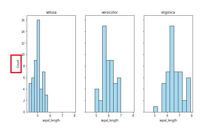
为了比较这三组的sepal_length有何不同之处，我们改采用 density方式图示之，如下图：

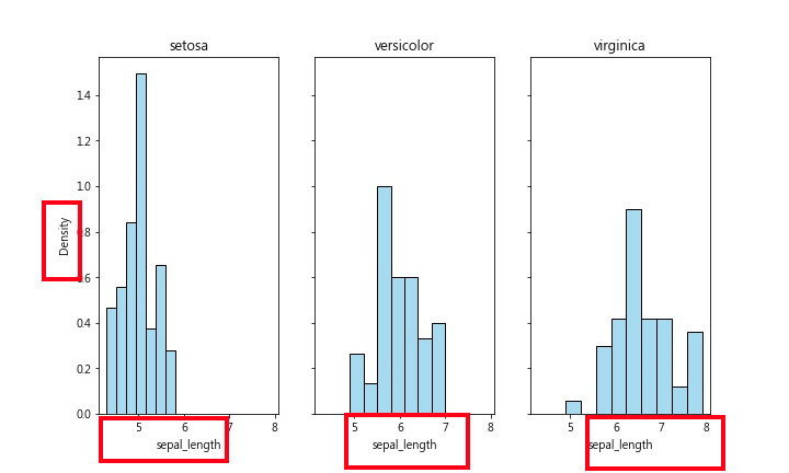
从此图可看出，setosa组大多数的sepal_length都比较小(小於6)，右边两图的数据大多数都是大於5。
三张图的bin 高度都是采用density表示
sns.histplot(color=,data= ,x=,ax=,stat=’density’)
从boxplot也可看出这种状况

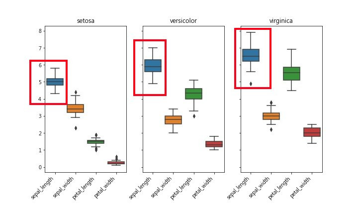
和上面使用EXCEL做出来的数据比对一下，也符合。

(三)、one-way ANOVA of python One-Way Analysis of Variances 单因子变异数分析
请参考这篇

先检查资料是否为常态分布
Perform the Shapiro-Wilk test for normality 参考此

指令 scipy.stats.shapiro(df0['sepal_length'])
返回两个数值ShapiroResult(statistic= , pvalue= )，第二个数字就是 p value，p >0.05是常态分布

''' Step 5.  check if Normal distribution   '''
import scipy.stats

def checkNS(vList):
    _,pValue = scipy.stats.shapiro(vList)
    return pValue

print(checkNS(df0['sepal_length']))
print(checkNS(df0['sepal_width']))

''' 略  '''

One-way ANOVA
Null hypothesis虚无假设：三个品种的”特徵平均值”，并无差异不同。
P 小於0.05 可推翻此null hypothesis
意思就是：三个品种的”特徵平均值”是不一样的。
表示：组间差异大於组内差异

''' Step 6. ANOVA test '''
dat0 = df0['sepal_length']
dat1 = df1['sepal_length']
dat2 = df2['sepal_length']

_,pANOVA = scipy.stats.f_oneway(dat0, dat1, dat2)

if pANOVA<=0.05:
    print('p value= %.6f '% pANOVA)

其它还有多项统计方法，下回再研究。

另外，要特别提醒的是，常常被误用的统计方法：Chi-square 并不适用於此数据集。
Chi-square 卡方检定应该运用於，多组样本之”次数统计”检定
请参考此

and here Chi-square

补充附记：
Seaborn relplot() 是一个资料视觉化的好用工具，一眼就可看出资料之关系/趋势。

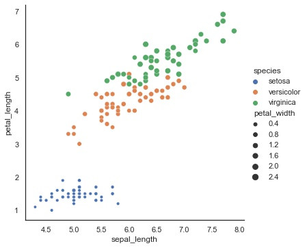
这张图可看出，三个品种从sepal_length (x轴)、petal_length (y轴)的scatter散点图，的确区分出三个不同群组。
使用hue参数表示三组。设定petal_width 给Size 点大的表示petal_width大
Virginica组的petal_width 都比较大

import seaborn as sns

sns.set_theme(style="white")

# Load iris dataset
iris = sns.load_dataset('iris')
iris.dropna(inplace=True)
print(iris.info())

sbplot = sns.relplot(x = 'sepal_length',
            y = 'petal_length',
            data = iris,
            kind = 'scatter',
            size = 'petal_width',
            hue = 'species')

sbplot.savefig('iris_scatter.jpg')