1　前言

近年来深度学习使用在许多比赛中，但几乎都使用ensemble(集成)的方式或是使用庞大的模型，这有个很严重的问题，那就是成本过高无法落地(除了原本就很昂贵的设备)，因此近几年也有许多人设计适用於嵌入式装置的模型，而Neural Architecture Search(NAS)便是解决办法之一，它能自动搜寻模型架构找到较为适合的架构，并且在效能上也能够有一定的表现，甚至有些NAS在训练时也能限制FPS和模型大小等等，如此一来在嵌入式装置也能够轻易地使用并且获得好的效能。

此篇文章要介绍的是Sequential Greedy Architecture Search(SGAS)[1]，SGAS是基於gradient descent(梯度下降演算法,GD)来找架构，这里我使用Convolutional neural network(CNN)作为范例 ，除了GS以外还有evolutionary algorithm (演化是演算法, EA)和reinforcement learning(强化学习,RL)等等方式能够找架构。想了解更多可参考AutoML Survey[2]。

2　SGAS贡献

首先简单的先了解SGAS的贡献。

1. 使用贪婪的方式进行剪枝。
2. 使用三种计算方式来定义剪枝的优先度，分别Edge Importance(重要性)、Selection Certainty(确定性)和Selection Stability(稳定性)三种计算来增加模型训练的稳定性。

3　SGAS演算法

3.1　Cell(Block)

注:假设Cell和Block是相同的东西
在开始进入SGAS时要先知道什麽是Cell(Block)，因为SGAS是在找出一个可能较好的Cell(Block)。这里使用Resnet[3]为例，我们常常会听到ResNet18/34/50/101/151...，而後面数字是代表经过了Ｎ层的运算层，其中运算层如卷积层和池化层等等，而Cell其实就是将几个运算层组合起来，如下图一(a)为ResNet-38的Cell，由此可知道ResNet-38是使用许多个Cell(a)所堆叠起来的网路，同理可知图一(b)也是一样，除此之外不同的Cell也会得到不同的效能。因此有许多人设计了不同的Cell来提升效能，而这篇论文是使用可微分与可加性来去找出最佳的Cell，如此一来能够因应不同的资料集并且减少人工设计的成本。

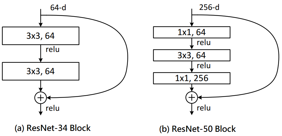
图一，来源[3]。

3.2　SGAS流程

从ResNet上面可以看到每一个箭头代表着一种运算层，而在SGAS中则是先定义N种运算层(3x3卷积层、最大池化层、5x5卷积层...)，也就是说第N层到第N+1层从原先只计算一个运算层变为需要计算N个运算层，如图二(a)，不同颜色的箭头代表着不同的运算层，而N个运算层会乘上一个对应的权重(训练出来的)做相加。

接着会先经过训练後，在N个运算层中选出一个较为重要的运算层，其余的则忽略，而这就是剪枝，如图二(b)，经过Greedy Decision在第0个节点和第1个节点选出蓝色线，再来经过训练後相同的经过Greedy Decision选择要剪枝的节点，如图二(c)，反覆此步骤直到每个节点都剪枝完毕，如图二(d)。

简单的例子：假设输入(1, 3, 32, 32)大小的资料。

• ResNet会输出是(1, 64, 32, 32)。
• 未剪枝的SGAS会有N个运算层则会变为[(1, 64, 32, 32), (1, 64, 32, 32)...N]，在乘上相对应的权重[0.1, 0.05...N]做加总，所以输出的大小一样是(1, 64, 32, 32)。
• 已剪枝的SGAS只会有一个运算层，所以输出的大小是(1, 64, 32, 32)。

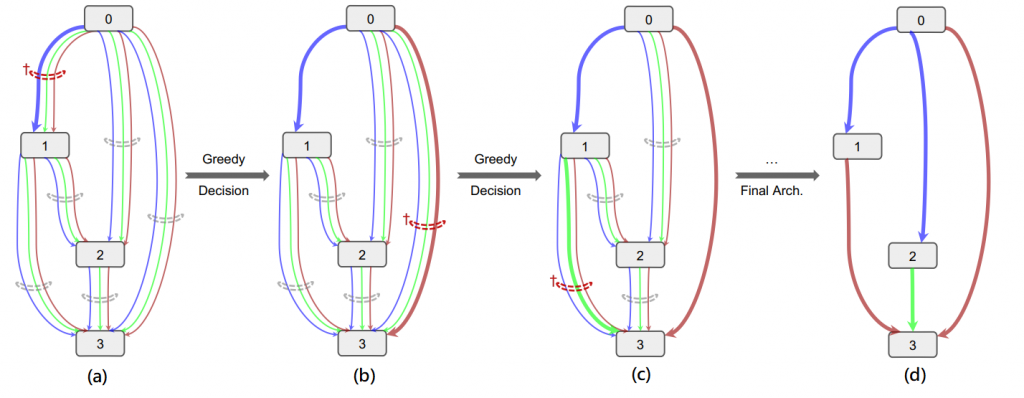
图二，来源[2]。

3.3　SGAS演算法

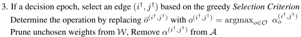
这里直接附上SGAS演算法，如图三，其中i和j代表着不同的节点，alpha代表运算层的重要度(权重)，W代表整体网路的权重，这里与上述的流程是相同的，只是用演算法的形式写出。

1. 使用验证集更新A(每一个alpha)。
2. 使用训练集更新W。
3. 经过Greedy Selection Criterion找出最大值的节点进行剪枝，剪枝过的alpha则不再更新。
   
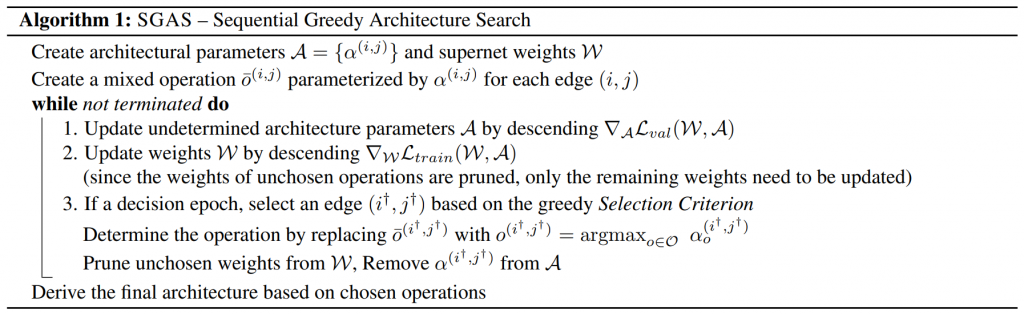
   图三，来源[2]。

3.3.1　Greedy Selection Criterion Formula

SGAS主要使用了三个公式作为Greedy Decision的选择标准。

• Edge Importance
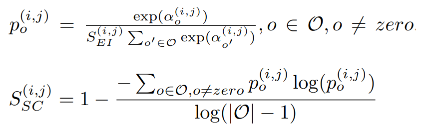
  第一个公式为计算alpha(i, j)的重要性，其中i、j为不同的节点。上述有提到每一次计算有N个运算层，而其中有一个运算层为non-zero层，也就是说经过non-zero层後的输出等於零，反向传播(偏微分)时的梯度一样为0，因此能够说如果alpha(i, j)的non-zero层的权重较大，代表着此层的重要程度是比较小的。详细公式如公式一。
  注:使用exp能将连乘的机率转为相加。

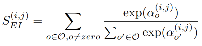
公式一，来源[2]。

• Selection Certainty
  第二个公式为计算alpha(i, j)的确定性，其中i、j为不同的节点。公式二则延续公式一，只是多使用entropy来计算平均的确定性。详细公式如公式二。
  这里举个简易的例子来看出entropy的特性，其中entropy公式为x*log(x)，可以看到越接近1或0的entropy都会比较大，因此能够利用entropy的特性来计算出不确定性(越接近0确定性越大)。而要计算确定性只要加上1即可。
  1.机率为0.9的entropy为0.9 * log(0.9) = -0.04，反之确定性=0.96。
  2.机率为0.1的entropy为0.1 * log(0.1) = -0.1，反之确定性=0.9。
  3.机率为0.5的entropy为0.5 * log(0.1) = -0.15，反之确定性=0.85。
  上述的例子可以得知0.5的不确定性较大，可以反应出未收敛或模型产生矛盾等等情况。
  注:计算一次极端状况能知道Selection Certainty是补足Edge Importance的不足。
  
  公式二，来源[2]。

• Selection Stability
  第二个公式为计算alpha(i, j)的稳定性，其中i、j为不同的节点。若只考虑公式一和公式二，可以知道两者仅仅只考虑当下的alpha(i, j)，这有可能会产生不稳定情形，例如第一次决策时的机率是0.1，第二次决策时的机率是0.9，第三次0.1，第四次0.9，这时就会有不稳定的情况，因此SGAS考虑了Ｔ个历史纪录，用来计算彼此的交集，这样能够将稳定度也考虑进去。详细公式如公式三。

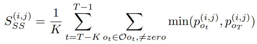
公式三，来源[2]。

3.3.2　Greedy Selection Criterion

SGAS使用了上述三个公式做评估，假设都是独立机率则相乘即可获得分数，而分数又分为Cri.1公式四和Cri.2公式五，差别在於有无考虑历史讯息(Selection Stability)。

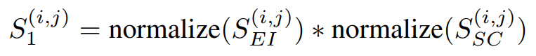
公式四，来源[2]。

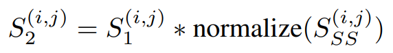
公式五，来源[2]。

4　主要程序码解析

4.1　Network

GitHub位置:/sgas/cnn/model_search.py

其它参数

一般的网路运算层基本上只有一个运算层，如3x3卷积层、5x5卷积层、3x3空洞卷积层....，而SGAS运算层定义为包含八种运算层，如下。

PRIMITIVES = [
    'none',
    'max_pool_3x3',
    'avg_pool_3x3',
    'skip_connect',
    'sep_conv_3x3',
    'sep_conv_5x5',
    'dil_conv_3x3',
    'dil_conv_5x5'
]

主要函数

MixedOp：当无选择的索引(未被剪枝)则计算八种运算层乘上权重的合，若有选择的索引(已剪枝)则选择该层运算做为输出。

class MixedOp(nn.Module):
    def forward(self, x, weights, selected_idx=None):
        if selected_idx is None:
            return sum(w * op(x) for w, op in zip(weights, self._ops))
        else:  # unchosen operations are pruned
            return self._ops[selected_idx](x)

Cell：SGAS用两个Node做为输入，分别是前一个Cell的输出(s0)，现在Cell的输出(s1)，这种想法其实有点类似ResNet和DenseNet，甚至未来可以尝试使用CSPNet的想法来减少计算量，而这里的**_steps表示操作次数，可以当作是Cell深度的上限(预设4)，每计算一次就可以得到更高阶的特徵，并且会将输出加入states list内以供下次操作使用，这里其实也隐含着类似ResNet和DenseNet**的想法，因为下一层还能够使用上一层的输入进行运算，可以让网路自行决定要使用低阶特徵或是高阶特徵。

注:这里特别的地方是states list的数量随着增加，但输出的数量是不变的，因为会将所有states list经过MixedOp的输出进行相加，这想法也就是特徵融合。

class Cell(nn.Module):
    def forward(self, s0, s1, weights, selected_idxs=None):
        s0 = self.preprocess0(s0)
        s1 = self.preprocess1(s1)

        states = [s0, s1]
        offset = 0
        for i in range(self._steps):
            o_list = []
            for j, h in enumerate(states):
                if selected_idxs[offset + j] == -1: # undecided mix edges
                    o = self._ops[offset + j](h, weights[offset + j])
                    o_list.append(o)
                elif selected_idxs[offset + j] == PRIMITIVES.index('none'): # pruned edges
                    continue
                else: # decided discrete edges
                    o = self._ops[offset + j](h, None, selected_idxs[offset + j])
                    o_list.append(o)
            s = sum(o_list)
            offset += len(states)
            states.append(s)

        return torch.cat(states[-self._multiplier:], dim=1)

Network _initialize_alphas:初始化每一个Cell内的运算层权重，与上述Cell回圈相同，而产生乱数的大小是运算层种类大小(8种运算)，而这里较为特别的地方是，分为alphas_normal和alphas_reduce权重，alphas_normal代表无需下采样的Cell，而alphas_reduce代表需要下采样的Cell，(部份研究)会分为两个区块的原因可能是下采样通常会设定不同的stride或池化层等等，因此这操作与无须下采样的Cell是稍微不同的，所以会分为两个区块进行。

Network forward:会先计算alphas权重，再呼叫Cell进行计算，与一般网路差别在於权重。

Network check_edges:在剪枝完後呼叫，会限制每一次操作(深度)，若以有max_num_edges个已决策的节点则其余节点可以忽略。这个函数在限制计算复杂度，而当限制越宽松(max_num_edges越大)则运算量越大与训练时间越久。

class Network(nn.Module):
    def _initialize_alphas(self):
        k = sum(1 for i in range(self._steps) for n in range(2 + i))
        num_ops = len(PRIMITIVES)

        self.alphas_normal = []
        self.alphas_reduce = []
        for i in range(self._steps):
            for n in range(2 + i):
                self.alphas_normal.append(Variable(1e-3 * torch.randn(num_ops).cuda(), requires_grad=True))
                self.alphas_reduce.append(Variable(1e-3 * torch.randn(num_ops).cuda(), requires_grad=True))
        self._arch_parameters = [
            self.alphas_normal,
            self.alphas_reduce,
        ]
        
    def forward(self, input):
        s0 = s1 = self.stem(input)
        for i, cell in enumerate(self.cells):
            if cell.reduction:
                selected_idxs = self.reduce_selected_idxs
                alphas = self.alphas_reduce
            else:
                selected_idxs = self.normal_selected_idxs
                alphas = self.alphas_normal

            weights = []
            n = 2
            start = 0
            for _ in range(self._steps):
                end = start + n
                for j in range(start, end):
                    weights.append(F.softmax(alphas[j], dim=-1))
                start = end
                n += 1

            s0, s1 = s1, cell(s0, s1, weights, selected_idxs)

        out = self.global_pooling(s1)
        logits = self.classifier(out.view(out.size(0), -1))
        return logits

    def check_edges(self, flags, selected_idxs, reduction=False):
        n = 2
        max_num_edges = 2
        start = 0
        for i in range(self._steps):
            end = start + n
            num_selected_edges = torch.sum(1 - flags[start:end].int())
            if num_selected_edges >= max_num_edges:
                for j in range(start, end):
                    if flags[j]:
                        flags[j] = False
                        selected_idxs[j] = PRIMITIVES.index('none') # pruned edges
                        if reduction:
                            self.alphas_reduce[j].requires_grad = False
                        else:
                            self.alphas_normal[j].requires_grad = False
                    else:
                        pass
            start = end
            n += 1

        return flags, selected_idxs

4.2　Architect

GitHub位置:/sgas/cnn/architect.py
Architect有使用到unrolled来控制是否要添加train data的hessian矩阵(梯度的方向)到优化器内，而这并不是该论文重点(预设false，其它dataset训练也无使用)，因此就先略过，有兴趣可找相关文献观看。

主要函数

使用validation data更新未剪枝的的alphas权重。(神经网路无更新)

class Architect(object):
  def _backward_step(self, input_valid, target_valid):
    loss = self.model._loss(input_valid, target_valid)
    loss.backward()

4.3　Train

GitHub位置:/sgas/cnn/train_search.py
现在知道主要的Network架构也知道验证更新参数时使用的是Architect，接着就是greedy decision的算法，这里就按照上述所讲的演算法和公式一步一步的讲解。

1.train

训练所对应的演算法就是1.使用validation data来更新alpha和2.使用train data来更新weights。

参数：
train_queue：train dataloader(Pytorch Class)
valid_queue：validation dataloader(Pytorch Class)
model：train model
architect：class of update alpha
input：train data
target：train target
input_search：validation data
target_search：validation target

def train(train_queue, valid_queue, model, architect, criterion, optimizer, lr, epoch):
    ...

        # Algorithm 1. Update undetermined architecture parameters(only alpha)
        architect.step(input, target, input_search, target_search, lr, optimizer, unrolled=args.unrolled)
        
        # Algorithm 2. Update weights W
        optimizer.zero_grad()
        logits = model(input)
        loss = criterion(logits, target)

    ...

2.edge_decision

注解对应到上述的公式1~5。演算法对应到3.剪枝，特别的是剪枝完还会使用model.check_edges检查已剪枝数量，以用来决定该层是否还需要剪枝(限制剪枝和运算量)。

参数：
args.use_history：用来决定要不要使用历史资料。
args.warmup_dec_epoch：能当做预训练(不做剪枝)。
args.decision_freq：剪枝频率。
candidate_flags：节点是否剪枝的标记。
score：将评估的标准经过正规化[0,1]相乘。
selected_edge_idx：取得最大分数的索引(贪婪算法)。
selected_op_idx：取得selected_edge_idx运算层机率最大的索引(贪婪算法)，因为前面忽略non-zero层所以这里index要+1转回原本运算层的index。

def edge_decision(type, alphas, selected_idxs, candidate_flags, probs_history, epoch, model, args):
    mat = F.softmax(torch.stack(alphas, dim=0), dim=-1).detach()
    
    # Formula 1
    importance = torch.sum(mat[:, 1:], dim=-1)

    # Formula 2
    probs = mat[:, 1:] / importance[:, None]
    entropy = cate.Categorical(probs=probs).entropy() / math.log(probs.size()[1])


    if args.use_history: # SGAS Cri.2 
        # Formula 3
        histogram_inter = histogram_average(probs_history, probs)
        probs_history.append(probs)
        if (len(probs_history) > args.history_size):
            probs_history.pop(0)
        
        # Formula 5
        score = utils.normalize(importance) * utils.normalize(
            1 - entropy) * utils.normalize(histogram_inter)

    else: # SGAS Cri.1
        # Formula 4
        score = utils.normalize(importance) * utils.normalize(1 - entropy)


    if torch.sum(candidate_flags.int()) > 0 and \
            epoch >= args.warmup_dec_epoch and \
            (epoch - args.warmup_dec_epoch) % args.decision_freq == 0:
        masked_score = torch.min(score,(2 * candidate_flags.float() - 1) * np.inf)
        selected_edge_idx = torch.argmax(masked_score)
        selected_op_idx = torch.argmax(probs[selected_edge_idx]) + 1 # add 1 since none op
        selected_idxs[selected_edge_idx] = selected_op_idx

        candidate_flags[selected_edge_idx] = False
        alphas[selected_edge_idx].requires_grad = False
        if type == 'normal':
            reduction = False
        elif type == 'reduce':
            reduction = True
        else:
            raise Exception('Unknown Cell Type')
        candidate_flags, selected_idxs = model.check_edges(candidate_flags,selected_idxs,reduction=reduction)
        print(type + "_candidate_flags {}".format(candidate_flags))
        score_image(type, score, epoch)
        return True, selected_idxs, candidate_flags

    else:
        print(type + "_candidate_flags {}".format(candidate_flags))
        score_image(type, score, epoch)
        return False, selected_idxs, candidate_flags

5.　结论

SGAS在NAS当中训练速度是相当快的，而这次只运行CNN，资料集使用Cifar-10和MNIST，但一般我们遇到的资料可能不是CNN，而SGAS也考虑的了这点，因此还能用於GCN等等上(其实满多都能用在不同地方)，另外如果有时间会在打上一篇来讲解如何用在Kaggle的铁达尼号或房价预测，并且使用sklearn-AutoML来进行比较，感觉上AutoML在节省人力与实用性算是相当高的，希望未来有机会能够在工作场所发挥。
有任何问题或笔误欢迎留言

6.　程序码

修改後原始码：jupyter notebook code
修改後原始码：Github
论文原始码：SGAS Github

7.　参考文献

[1] Li, G., Qian, G., Delgadillo, I.C., M¨uller, M., Thabet, A., Ghanem, B.: Sgas: Sequential greedy architecture search. In: Proceedings of the IEEE Conference on
Computer Vision and Pattern Recognition (2020).
[2] X. He, K. Zhao, and X. Chu, “Automl: A survey of the state-of-the-art,” arXiv preprint arXiv:1908.00709 (2019).
[3] K. He, X. Zhang, S. Ren, and J. Sun. Deep residual learning for image recognition. In CVPR, 2016.