Day23 - 静态模型 part1 (MLP)
完整的语音情绪辨识系统流程如图 1。语音讯号先经过特徵撷取的过程撷取出声学特徵,再将声学特徵进行前处理,经过前处理过後的特徵做为分类模型的输入并进行训练。分类模型训练完成之後,再将测试资料输入至分类模型中得到分类结果。
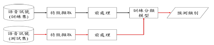
图 1: 语音辨识系统流程图。黑色箭头表示训练阶段,红色箭头表示测试阶段
实验中超参数(hyper-parameter)的设定是根据 early-stopping 演算法,我们将原始训练集的 80% 做为训练集而剩余的 20% 做为 early-stopping 演算法需要的验证集(validation set)。当训练过程中每一个 epoch 结束时,如果验证集的损失获得改善我们就会储存此次 epoch 的模型参数,当连续 patience 次的训练与已纪录的最佳验证集损失相比都没有改善的话,训练就会结束。训练结束时最後回传的会是最佳的模型参数(验证集损失最佳)。
在训练神经网路时设定的超参数如表 1,其中,optimizer的部份采用 adam 与 sgd,主要的差别在於训练过程中 adam 的收敛速度较快,因此训练次数会较少;而 sgd 收敛速度较慢,因此训练次数会较多。
| hyper-parameter | value |
|---|---|
| mini-batch | 100 |
| learning rate | 0.002 |
| learning rate decay | 0.00001 |
| optimizer | (1) adam (2) sgd |
| loss function | cross-entropy |
| patience | 3 |
表 1: 模型超参数
learning rate decay 的公式如下:
首先先对静态模型进行说明,我们会采用 MLP (Multilayer Perceptron) 与 CNN 两种架构。
MLP 的架构如下图 2:
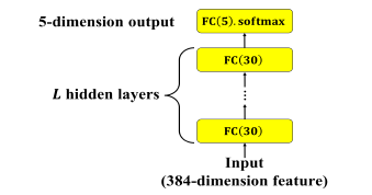
图 2: MLP 静态模型。L 表示隐藏层层数
输入为 Day20 时说明过的 384 维的特徵向量,隐藏层为 30 个神经元并采用两种 activation function (tanh、ReLU) 的全连接层 (Fully Connected, FC),共有 L 层,输出层为 5 个神经元的全连接层,activation function为 softmax。不同层数与不同激活函数的实验结果比较如表 2。
Activation function 参考:https://himanshuxd.medium.com/activation-functions-sigmoid-relu-leaky-relu-and-softmax-basics-for-neural-networks-and-deep-8d9c70eed91e
| hidden layers (L) | UA recall (tanh) | UA recall (ReLU) |
|---|---|---|
| 1 | 46.0% | 45.5% |
| 2 | 46.2% | 45.9% |
| 3 | 45.9% | 45.4% |
表2: 不同层数及不同activation function MLP 结果比较
从表中可发现网路架构的深度与 UA recall 并非成正比关系,两层隐藏层的表现要比三层来的更好。主要原因应为训练集的资料量并不多,因此如果模型复杂度太高反而会使模型在训练集上产生过拟合(overfitting)的现象。
程序的部分如下:
import os
os.environ['TF_CPP_MIN_LOG_LEVEL'] = '3'
import tensorflow as tf
import numpy as np
import argparse
import math

from keras.layers import *
from keras.models import *
from keras.optimizers import SGD, Adam
from keras.callbacks import EarlyStopping, ModelCheckpoint
from keras.layers.merge import *
from utils import *
from keras import backend as K
from keras.models import load_model
from keras.utils import plot_model, print_summary

MODEL_ROOT_DIR = './static_model/'

# Learning parameters
BATCH_SIZE = 100
TRAIN_EPOCHS = 10
LEARNING_RATE = 0.002
DECAY = 0.00001
MOMENTUM = 0.9
# Network parameters
CLASSES = 5 # A,E,N,P,R
LLDS = 16
FUNCTIONALS = 12
DELTA = 2
STATIC_FEATURES = LLDS*FUNCTIONALS*DELTA
HIDDEN_UNITS = 30
USE_TEACHER_LABEL = 0


def train_MLP(train_data, train_label, train_size, test_data, test_label, test_size):
	args = get_arguments()
	data_weights = []
	data_weights.append([1.1,0.5,0.2,1.5,1.4])
	data_weights = np.asarray(data_weights)
	class_weight = {0: 1.1, 1: 0.5, 2: 0.2, 3: 1.5, 4: 1.4}

	# 16x12x2
	mlp_input = Input(shape=[args.static_features], dtype='float32', name='mlp_input')
	hidden_1 = Dense(units=30, activation='relu', name='hidden1')(mlp_input)
	hidden_2 = Dense(units=30, activation='relu', name='hidden2')(hidden_1)
	hidden_3 = Dense(units=30, activation='relu', name='hidden3')(hidden_2)
	output = Dense(units=5, activation='softmax', name='output')(hidden_3)
	model = Model(inputs=mlp_input, outputs=output)
	model.summary()

	if args.load_model == '':
		adam = Adam(lr=args.learning_rate, decay=args.decay)
		model.compile(loss=weighted_loss(r=data_weights), optimizer=adam, metrics=['accuracy'])
		earlystopping = EarlyStopping(monitor='loss', min_delta=0, patience=0)
		checkpoint = ModelCheckpoint(filepath='static_model/mlp_checkpoint.hdf5', monitor='val_loss', save_best_only=True)
		callbacks_list = [earlystopping, checkpoint]
		history = model.fit(x=train_data, y=train_label, batch_size=args.batch_size, epochs=args.train_epochs, verbose=2,
							  callbacks=callbacks_list)
		# save the model
		model.save_weights(args.model_root_dir + 'model.h5')
	else:
		print ('Load the model: {}'.format(args.load_model))
		model.load_weights(args.model_root_dir + args.load_model)

	predict = model.predict(test_data, verbose=1)
	show_confusion_matrix(predict, test_label, test_size)
在後续的模型中,我们会针对分类结果较好的其中几个模型列出混淆矩阵(confusion matrix)来详细观察各类别的分类情形。
画出 confusion matrix 的程序如下:
def show_confusion_matrix(predict, true_label, size):
	num_class = true_label.shape[1]
	AC = np.zeros(num_class)# store the classification result of each class
	AC_WA = 0.0
	AC_UA = 0.0
	confusion_matrix = np.zeros((num_class, num_class))# store the confusion matrix

	for i in range(predict.shape[0]):
		predict_class = np.argmax(predict[i])
		true_class = np.argmax(true_label[i])
		confusion_matrix[true_class][predict_class] += 1
	for i in range(num_class):
		AC[i] = confusion_matrix[i][i] / size[i]

	print("-------------Classification results-------------")
	print ('A: {0} , E: {1} , N: {2} , P:{3} , R: {4}'.format(size[0],size[1],size[2],size[3],size[4]))
	AC_UA = np.mean(AC)
	AC_WA = (confusion_matrix[0][0] + confusion_matrix[1][1] + confusion_matrix[2][2] + confusion_matrix[3][3] + confusion_matrix[4][4] ) / predict.shape[0]
	print('      A      E      N      P      R')
	print('A  %4d   %4d   %4d   %4d   %4d    ' % (confusion_matrix[0][0], confusion_matrix[0][1], confusion_matrix[0][2], confusion_matrix[0][3], confusion_matrix[0][4]))
	print('E  %4d   %4d   %4d   %4d   %4d    ' % (confusion_matrix[1][0], confusion_matrix[1][1], confusion_matrix[1][2], confusion_matrix[1][3], confusion_matrix[1][4]))
	print('N  %4d   %4d   %4d   %4d   %4d    ' % (confusion_matrix[2][0], confusion_matrix[2][1], confusion_matrix[2][2], confusion_matrix[2][3], confusion_matrix[2][4]))
	print('P  %4d   %4d   %4d   %4d   %4d    ' % (confusion_matrix[3][0], confusion_matrix[3][1], confusion_matrix[3][2], confusion_matrix[3][3], confusion_matrix[3][4]))
	print('R  %4d   %4d   %4d   %4d   %4d    ' % (confusion_matrix[4][0], confusion_matrix[4][1], confusion_matrix[4][2], confusion_matrix[4][3], confusion_matrix[4][4]))
	print('\nA: %f    E: %f     N: %f     P: %f     R: %f\n' % (AC[0]*100, AC[1]*100, AC[2]*100, AC[3]*100, AC[4]*100))
	print("WA: {}".format(AC_WA*100))
	print("UA: {}".format(AC_UA*100))
	print("------------------------------------------------")
明天将继续介绍静态模型-CNN 部分。
>>: Day19【Web】网路攻击:网路钓鱼(Phishing)
Day17:今天来聊一下如何使用macof产生MAC Flooding
MAC Flooding是一种用於危及连接网段或网络设备的网路Switch安全技术。 攻击者使用MA...
电子书阅读器上的浏览器 [Day18] 支援夜间模式
夜间模式在电子书阅读器上通常效果不会很好,黑色的底色会造成很多残影。不过,因为我也会在一般手机上使用...
Day6 Let's ODOO: Model(3) Decorators & Environment
依照昨天范例我们继续写下去 # -*- coding: utf-8 -*- from odoo im...
【Aspose系列】Aspose.Cells (1) - 建立/读取Workbook、WorksheetCollection
这个系列旨在介绍 Aspose 的几类常用 API,有兴趣的话就一起往下看吧!此系列中不会包含 As...
Day30 - 导入 Next.js 的杂谈与系列文总结
尾声 最後一天想回归到第一天时对自己说的话「看完这些文章的读者能够对 Next.js 有更多的了解,...