[神经机器翻译理论与实作] 你只需要专注力(III): 建立更专注的seq2seq模型（续曲）

前言

今天我们将稍微讲述 Luong 全域注意力机制的原理，并继续用 Keras 来架构附带注意力机制的 seq2seq 神经网络。

Luong Attention

Luong attention 机制分为全域（ global ）和局部（ local ）两种策略：

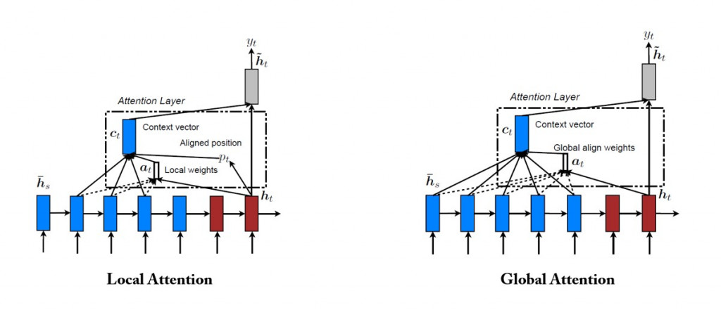
我们采用全域 Luong attention 机制：

回归注意力机制的本质: Query, Keys, and Values

记忆上下文关系的 context vector 为各个单词的加权平均，其中注意力权重（或称词权重）为当下解码器内部状态 与各个单词向量 之间关联分数出现之机率：

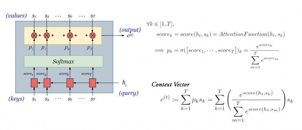
而在前天的文章里，我们提过三种常见的 attention functions ，今天我们将采用最简单的点积法。

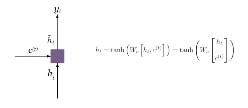
从context vector到解码器输出词向量

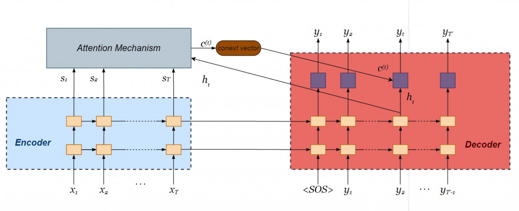
对比附带注意力机制的编码器则在遍历所有的时间点之後仅输出单一个 context vector ，注意力机制则是针对当下时间点产出 context vector ，每个时间点的 context vector 会不断更新，有效采计较遥远的历史资讯。将解码器当下的内部状态和 context vector 连接在一起（ concatenate ），经过线性转换 之後，再经过激活函数 （ hyperbolic tangent ），产生专注向量（ attentional vector ） ，是为 Luong 注意力机制的输出向量。

图片来源：https://memes.tw/

你以为事情就这样结束了吗？我们还没得到解码器最终的输出值 呢！为了预估当下最有可能出现的单词，我们还需要透过 softmax 分派机率值到目标语言 word embedding 的各个维度。以下为解码器的最终步骤：在已知完整来源语言序列 和过往翻译单词 的条件下，当下输出值 出现的条件机率。

理论言毕，接着我们将 Luong （全域）注意力机制加入昨天建构好的双层 LSTM Encoder-Decoder 网络。

用Keras建立注意力层神经元（下篇）

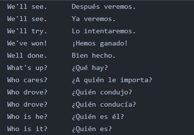
我们延续Seq2Seq 实作第一篇 的情境，使用以下的英文－西班牙文（双语）平行语料库：

超参数设定

来源语言（英文）的词向量维度是18（为了方便解说我们使用了 one-hot 编码，而实务上多用 word2Vec 生成 word embedding ），含有标点符号句长最大值为 4；目标语言（西班牙文）的词向量则为27，含有句子起始符号 <SOS> 及终止符号 <EOS> 的句长最达值为12。 LSTM 的内部状态为 256维的向量。我们按照此指定超参数：

### preparing hyperparameters

## source language- English
src_wordEmbed_dim = 18 # dim of text vector representation
src_max_seq_length = 4 # max length of a sentence (including punctuations)

## target language- Spanish
tgt_wordEmbed_dim = 27 # dim of text vector representation
tgt_max_seq_length = 12 # max length of a sentence (including <SOS> and <EOS>)

# dim of context vector
latent_dim = 256

编码器微调

与昨天的编码器设定大致一样，唯一不同之处为我们需要将编码器最上层的输出值（其实就是各个 LSTM 小单元的 hidden state ）传入注意力层，因而将第二层 LSTM 设定 return_sequences = True 。

### Building a 2-layer LSTM encoder
enc_layer_1 = LSTM(latent_dim, return_sequences = True, return_state = True, name = "1st_layer_enc_LSTM")
# set return_sequence to True so that encoder outputs can be input to attention layer
enc_layer_2 = LSTM(latent_dim, return_sequences = True, return_state = True, name = "2nd_layer_enc_LSTM")
enc_inputs = Input(shape = (src_max_seq_length, src_wordEmbed_dim))
enc_outputs_1, enc_h1, enc_c1 = enc_layer_1(enc_inputs)
enc_outputs_2, enc_h2, enc_c2 = enc_layer_2(enc_outputs_1)
enc_states = [enc_h1, enc_c1, enc_h2, enc_h2]

解码器微调

由於我们将当下的内部状态 当作 query 传入注意力层，先删除原有用来预估当下输出的激活函数 softmax 。而最上层的 LSTM 也不必回传内部状态，因此设定 return_state = False 。

### Building a 2-layer LSTM decoder
dec_layer_1 = LSTM(latent_dim, return_sequences = True, return_state = True, name = "1st_layer_dec_LSTM")
dec_layer_2 = LSTM(latent_dim, return_sequences = True, return_state = False, name = "2nd_layer_dec_LSTM")
dec_dense = Dense(tgt_wordEmbed_dim, activation = "softmax")
dec_inputs = Input(shape = (tgt_max_seq_length, tgt_wordEmbed_dim))
dec_outputs_1, dec_h1, dec_c1 = dec_layer_1(dec_inputs, initial_state = [enc_h1, enc_c1])
dec_outputs_2 = dec_layer_2(dec_outputs_1, initial_state = [enc_h2, enc_c2])

注意力层

首先是计算关联性分数（ attention score ）

from tensorflow.keras.layers import dot

attention_scores = dot([dec_outputs_2, enc_outputs_2], axes = [2, 2])

接着算出注意力权重

from tensorflow.keras.layers import Activation

attenton_weights = Activation("softmax")(attention_scores)
print("attention weights - shape: {}".format(attenton_weights.shape)) # shape: (None, enc_max_seq_length, dec_max_seq_length)

利用加权平均求出context vector

context_vec = dot([attenton_weights, enc_outputs_2], axes = [2, 1])
print("context vector - shape: {}".format(context_vec.shape)) # shape: (None, dec_max_seq_length, latent_dim)

将解码器当下的内部状态与context vector连接起来，并得到注意力层的输出

# concatenate context vector and decoder hidden state h_t
ht_context_vec = concatenate([context_vec, dec_outputs_2], name = "concatentated_vector")
print("ht_context_vec - shape: {}".format(ht_context_vec.shape)) # shape: (None, dec_max_seq_length, 2 * latent_dim)

# obtain attentional vector
attention_vec = Dense(latent_dim, use_bias = False, activation = "tanh", name = "attentional_vector")(ht_context_vec)
print("attention_vec - shape: {}".format(attention_vec.shape)) # shape: (None, dec_max_seq_length, latent_dim)

传入softmax层预估当下输出值的条件机率

将注意力机制的输出值传入 softmax 层得到当下的目标词向量：

dec_outputs_final = Dense(tgt_wordEmbed_dim, use_bias = False, activation = "softmax")(attention_vec)
print("dec_outputs_final - shape: {}".format(dec_outputs_final.shape)) # shape: (None, dec_max_seq_length, tgt_wordEmbed_dim)

全部整合起来！

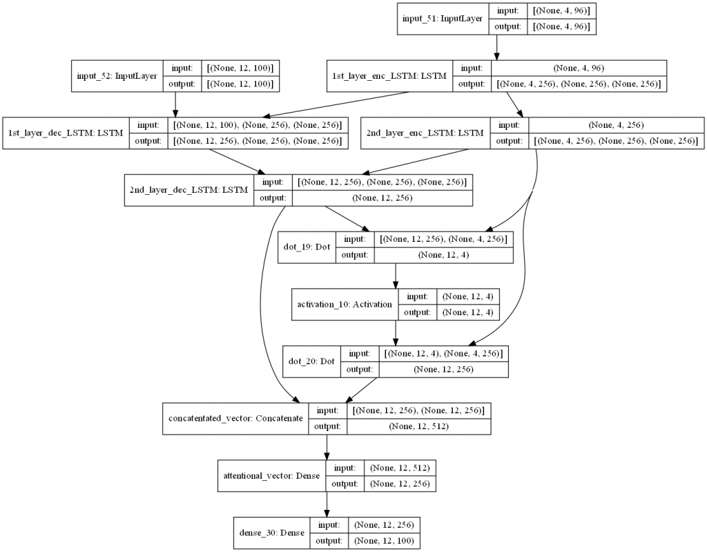
我们使用 tf.keras.models.Model 物件，指定模型的输入（与未附加注意力机制的 seq2seq 相通）与模型的输出，将 encoder 、 decoder 以及 attention layer 三者串连起来，并使用 plot_model 函式画出模型的架构：

from tensorflow.keras.utils import plot_model

# Integrate seq2seq model with attention mechanism
seq2seq_2_layers_attention = Model([enc_inputs, dec_inputs], dec_outputs_final, name = "seq2seq_2_layers_attention")
seq2seq_2_layers.summary()

# Preview model architecture
plot_model(seq2seq_2_layers_attention, to_file = "output/2-layer_seq2seq_attention.png", dpi = 100, show_shapes = True, show_layer_names = True)

结语

以上我们示范了如何利用 Keras API 建构出附带 Luong 全域注意力机制的 LSTM seq2seq 的神经网络。由於时间有限，我们得先停在这里，而仍有以下残留课题：

• 使用物件导向设计编码器、解码器以及注意力层之类别
• 比较来源词句与目标词句的关联性

各位有个美好的周末吗？我们明天见！

阅读更多

1. Attention Mechanism
2. keras的几种attention layer的实现之一 | 知乎