[神经机器翻译理论与实作] Google Translate的神奇武器- Seq2Seq (II)

前言

我们紧接着切入 RNN 为架构的编码器-解码器。

在seq2seq之前

RNN Encoder-Decoder

在 Google 正式提出 seq2seq 架构之前， Cho 等人就提出了以标准循环神经网络（ standard RNN ）设计编码器-解码器的演算法：

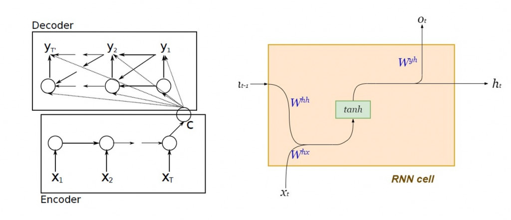
图片来源：Learning Phrase Representations using RNN Encoder–Decoder for Statistical Machine Translation

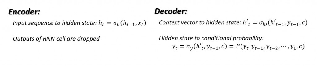
编码器及解码器内部的动态系统方程：

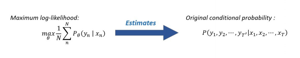
其用意是为了以最大似然（ maximum likelihood ）估计来条件机率：

单层LSTM Encoder-Decoder

最简单的 seq2seq 编码器内部由一层 LSTM 细胞串联而成，下图右方为每个 LSTM 细胞内部的结构以及其动态方程：

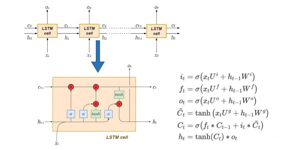
虽然传统 RNN 的内部隐藏状态（ hidden state ）能够保存上下文关系，然而在输入的单词序列过长时，距离预测愈遥远的历史讯息几乎已无发挥影响力，将会发生梯度消失（ vanishing gradient ），在长句的翻译上未能达到令人满意的效果。而 LSTM 保留了 RNN 原有的隐藏状态，并加入了细胞状态（ cell state ）来记录距离预测值遥远的历史资讯，以实现长期依赖（ long-term dependency ）。

Hidden state捕捉短期记忆，而cell state则储存长期记忆：
Characterization is an abstract term that merely serves to illustrate how the hidden state is more concerned with the most recent time-step. The cell state is basically the global or aggregate memory of the LSTM network over all time-steps.

文字出处：LSTMs Explained: A Complete, Technically Accurate, Conceptual Guide with Keras

写一个简单的seq2seq网络吧

接下来我们将使用 Tensorflow 建立单层的 LSTM seq2seq 。在这里我们先示范如何利用 Keras API 的模型定义编码器及解码器，而不细谈文本的来源与文字前处理，以及如何直接使用 Tensorflow 基本语法建立 seq2seq 模型。

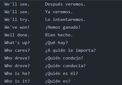
我们以翻译作为前提，考虑意义相同的来源语言文句以及目标语言文句并行条列而成的双语平行文本（如下图所示）：

资料准备

首先要确立的是编码器输入资料的张量维度「 来源语言文句总数 × 来源语言中最长文句之词条数量 × 来源语言内撇除重复词条的总数 」，并指定资料型态为单精确浮点数 float32：

import numpy as np
from preprocess_text import input_docs, target_docs, input_tokens, target_tokens, num_encoder_tokens, num_decoder_tokens, max_encoder_seq_length, max_decoder_seq_length

encoder_input_data = np.zeros(
    shape = (len(input_docs), max_encoder_seq_length, num_encoder_tokens),
    dtype = "float32"
    )

接下来确立解码器输入资料的张量维度「 来源语言文句总数 × 目标语言最长文句之词条数量 × 目标语言内撇除重复词条的总数 」以及输出资料的张量维度「 目标语言文句总数 × 目标语言最长文句之词条数量 × 目标语言内撇除重复词条的总数 」

# Build out the decoder_input_data matrix:
decoder_input_data = np.zeros(
    (len(input_docs), max_decoder_seq_length, num_decoder_tokens),
    dtype = "float32"
    )
# Build out the decoder_target_data matrix:
decoder_target_data = np.zeros(
    (len(target_docs), max_decoder_seq_length, num_decoder_tokens),
    dtype = "float32"
    )

接下来将单词表示为向量，并依照前後顺序（建立时间序列），填入刚才建立的 NumPy 阵列！虽然在实务应用上，翻译任务的词汇表通常极为庞大，往往使用word2Vec 进行 word embedding 到相对低维度的向量，但在这里我们采用 one-hot 编码，因此单词向量之维度便是文本词汇量。

# since we're using a bilingual parallel corpus, we have the same number of sentences in both languages, therefore same size of input and target documents
for line, (input_doc, target_doc) in enumerate(zip(input_docs, target_docs)):
    for timestep, token in enumerate(re.findall(r"[\w']+|[^\s\w]", input_doc)):
        encoder_input_data[line, timestep, input_features_dict[token]] = 1.
    for timestep, token in enumerate(target_doc.split()):
        decoder_input_data[line, timestep, target_features_dict[token]] = 1.
        if timestep > 0:
            decoder_target_data[line, timestep - 1, target_features_dict[token]] = 1.

今天的介绍就先写到这里，明天继续！

阅读更多

1. Learning Phrase Representations using RNN Encoder-Decoder for Statistical Machine Translation
2. Keras API- LSTM