Chap.II Machine Learning 机器学习

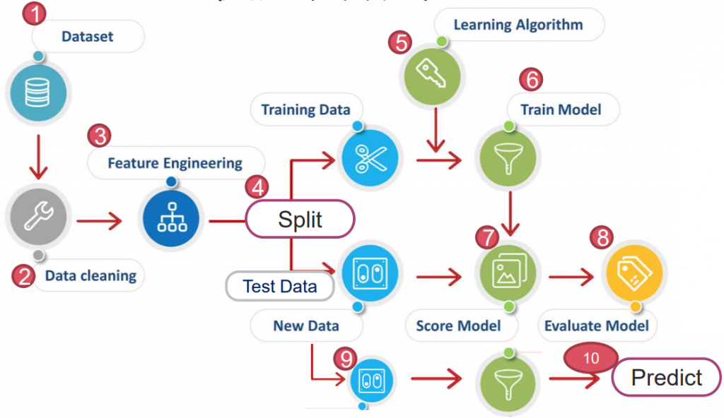
https://yourfreetemplates.com/free-machine-learning-diagram/

Part 1：Exploratory Data Analysis 资料探索与分析

Exploratory Data Analysis 又称 EDA。
为了解资料的主要特性，会将蒐集而来的资料作分析，且常采用视觉化来进行判断。
狭义来说，EDA 即资料收集/资料处理/视觉化...等过程。广义来说，EDA 还包含 Data Clean。

1. Dataset（资料探索）：
2. Data Clean（资料清洁）：对资料进行一定程度的清洁，去除无项目项次、填满或补 0 等。
   *一般机器学习过程中，资料探索与清洁是会交互处理的，会重复几次甚至几百次，直至获取有意义的资料集。

1-1. Dataset 资料集

基本资料的汇入、找寻。纯粹做练习用的资料如下：

1. UCI及其他套件（如：Scikit-Learn、Seaborn、StatsModels...等）
2. Kaggle　*世界最有名的资料竞赛
3. Goole Dataset search
4. 政府部门资料

1-2. Data Clean 资料清洁

常包含以下几个步骤：

1. Merge 合并资料
2. Rename 重新命名栏位名称
3. Missing Value 遗失值
4. Transform column Data Type 资料类型转换
5. Feature Engineering and Transforming Variables 特徵工程与变数转换
6. Transform Numeric Variables 转换数值变数
7. Remove Duplicate rows 移除重复值

1-3. Visualization 视觉化

常用的指令有几种，包含 matplotlib(*补充看我、或我)、pandas 中的 plot 以及 seaborn(*补充看我)...等。

以下会以"tips"资料集来介绍 seaborn 的几种图：

# 载入必要套件 & 'tips' 资料集
import numpy as np
import pandas as pd
import matplotlib.pyplot as plt
import seaborn as sns
tips = sns.load_dataset('tips')

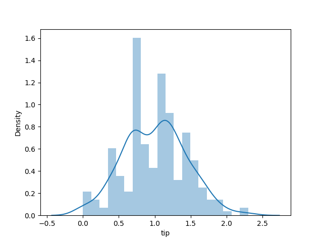
1. 直方图 sns.distplot：呈现单变数（也可用 histplot，但就没有偏移曲线）

# 通常偏移分配，会多取 log 矫正
sns.distplot(np.log(tips['tip']), bins=20) # , kde=False

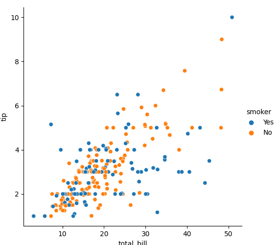
2. 关系散部图 sns.relplot：用在 x y 关系为相对(另一绝对散部图见补充 1.)

# hue= : 可以依照选择 item 以颜色区分
sns.relplot(x='total_bill', y='tip', data=tips, hue='smoker')

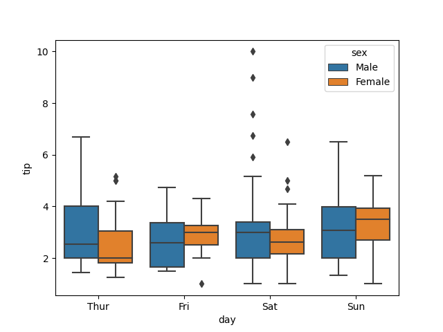
3. 盒需图 sns.boxplot

sns.boxplot(x='day', y='tip', data=tips, hue='sex')

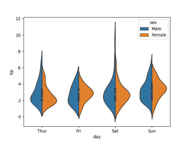
4. 小提琴图 sns.violinplot

# split=True：可将 hue 的内容分布在两侧
sns.violinplot(x='day', y='tip', data=tips, hue='sex', split=True)

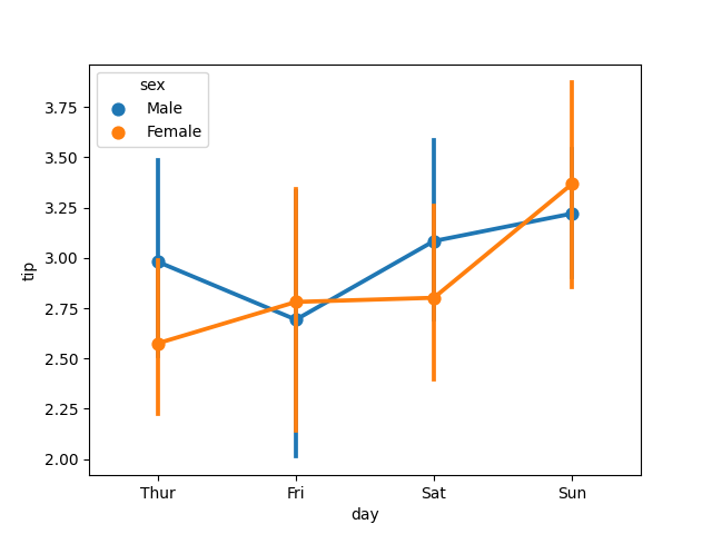
5. 点图 sns.pointplot

sns.pointplot(x='day', y='tip', data=tips, hue='sex')

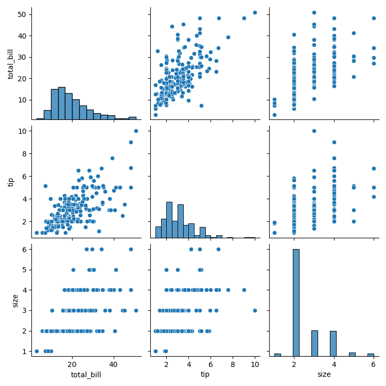
6. 配对图 sns.pairplot：把各个 item 配对成散部图

sns.pairplot(tips)

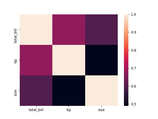
7. 热力图 sns.heatmap：把各个 item 配对，依照影响权重上色

sns.heatmap(tips.corr())

看完以上，接着用经典范例-铁达尼号 来操作 EDA：

1. Import tools & Load data

import pandas as pd
import seaborn as sns

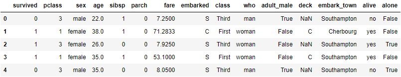
df = sns.load_dataset('titanic')
df.head(10)

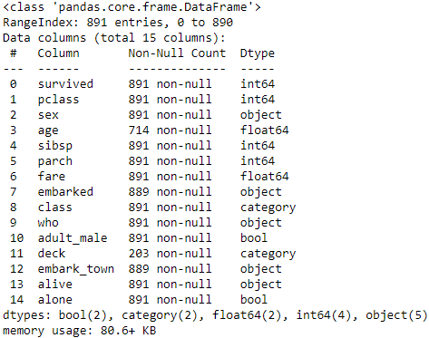
查看资料类型

df.info()

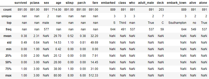
查看描述统计量

df.describe(include='all')

2. Analysis Y (此例中为'survived')

df['survived'].nunique()
>>  2

df['survived'].unique()
>>  array([0, 1], dtype=int64)

df['survived'].value_counts()
>>  0    549
    1    342
    Name: survived, dtype: int64

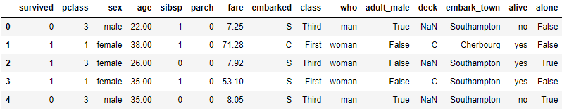
3. Deal w/ NaN value

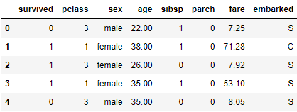
# initial data
df.head()

# check NaN value
df.isna().sum()

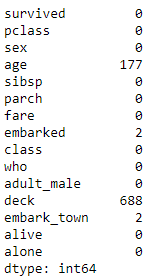
可以发现有许多重复/缺失项目，下面一项一项来处理：

A. 删去重复项目

df.drop(['who', 'deck', 'embark_town','adult_male', 'deck', 'class', 'alive', 'alone'],
    axis=1, inplace=True)
df.head()

B. 填补缺失项目
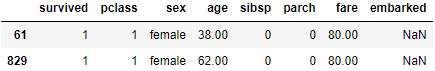
B-1. 填补 age

df[df['age'].isna()]

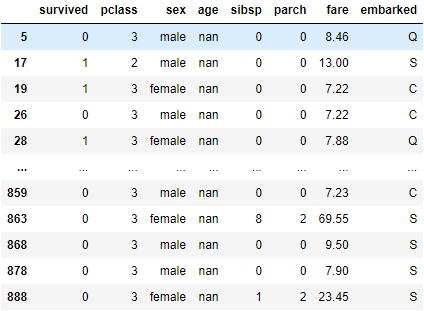
# 使用中位数来填补
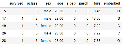
df['age'].fillna(df['age'].median(), inplace=True)
df.iloc[[5, 17, 19, 26, 28]]   # 挑其中几个检查

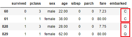
B-2. 填补 embarked

df[df['embarked'].isna()]

# 以前面一个的值填补
df['embarked'].fillna(method='ffill', inplace=True) # 或者 method='bfill'
df.iloc[[60, 61, 828, 829]]

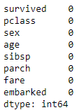
*Double check

df.isna().sum()

4. 转换非数字资料

有序 ordinal: 特徵值隐含顺序及大小高低之分 如: 'class' 'age' 等
名目 nominal: 不含顺序大小 如: 'sex' 'embarked'
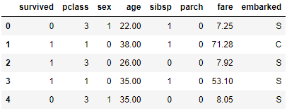
A. 将 'sex' 转换为 0/1

df.sex.unique()
>>  array(['male', 'female'], dtype=object)

df.sex = df.sex.map({'male':1, 'female':0})
df.head()

B. 将 'embarked' 转换

# 确认登船港口 vs. 生存率
sns.barplot(data=df, x='embarked', y='survived')

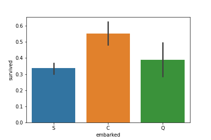
根据史料，登船港口依序为 Southampton -> Cherbourg -> Queenstown
此结果显示登船港口与生存率无显着相关，并没有因为早上船而容易死亡。
故将其转换为 one-hot encoding，避免影响判断。

df.embarked.unique()
>>  array(['S', 'C', 'Q'], dtype=object)

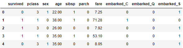
# Transfer
df = pd.get_dummies(df, columns=['embarked'])
df.head()

C. 将年龄转换为级距
因考虑各个年龄层生存机率应相近，故使用 pd.cut() 将 'age' 切成几个级距。
首先观察各个级距存活率：

bins=[0, 12, 22, 30, 50, 60, 100]
age_cut = pd.cut(df['age'], bins)

sns.barplot(x=age_cut, y=df['survived'])

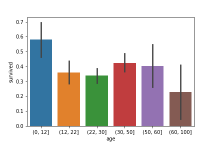
依据上图，将各个年龄层进行有序 (ordinal) 编码。生存机率最高为 5；最低为 0。

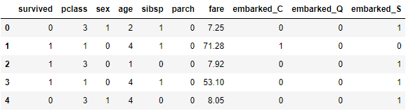
df['age'] = pd.cut(df['age'], bins, labels=[5, 2, 1, 4, 3, 0])
df.head()

D. 归一化 'fare'
找出票价为 0 者：

df[df['fare'] == 0]

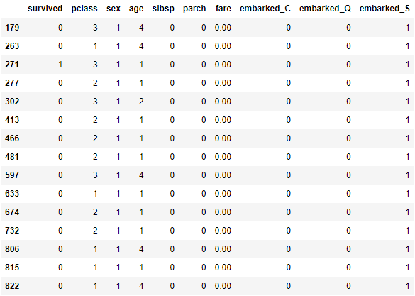
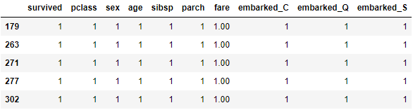
重设票价 0 为至少 1 块钱：

df[df['fare'] == 0] = 1
df.iloc[[179,  263, 271, 277, 302]]

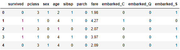
归一化：

import numpy as np
df['fare'] = np.log(df['fare'])
df.head()

5. Analize relationship between X & Y

资料整理完成後 方可确认各个资讯间的关联，以下用热力图做范例：

sns.set(style='ticks', color_codes=True)
plt.figure(figsize=(14, 12))
sns.heatmap(df.corr(), linewidths=0.1, square=True, linecolor='w', annot=True)
plt.show()

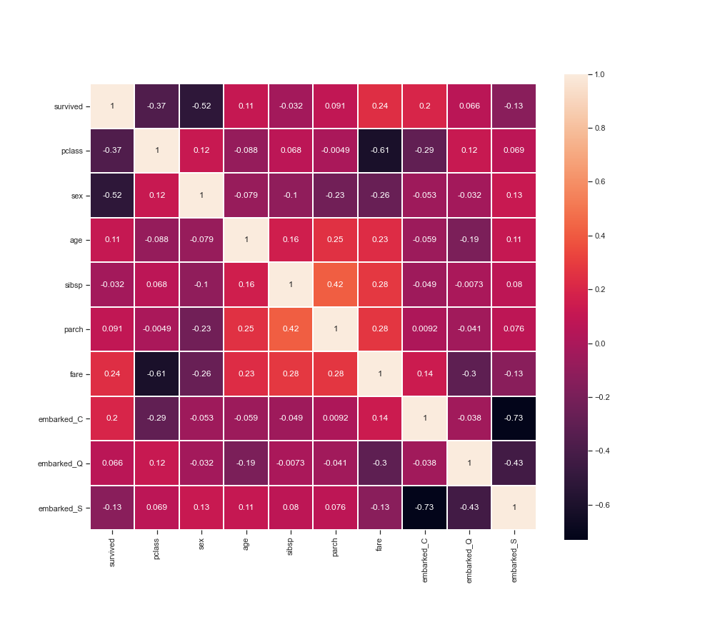
从以上分析可知：生存机率与舱等、性别高度相关。

6. Split Data

from sklearn.model_selection import train_test_split
y = df['survived']
X = df.drop('survived', axis=1)

X_train, X_test, y_train, y_test = train_test_split(X, y, test_size=0.2)

7. Feature Scaling (Normalization or Standardization)

为使收敛速度加快，通常在切割资料後会进行以下步骤其一：

1. 正规化 Normalization: 将资料等比例缩放到 [0, 1] 区间中。
   X_nor = (X - Min)/(Max-Min)
2. 标准化 Standardization: 将资料经 Z 转成标准常态分布 (Standard Normal Distribution)，即 X 距离 mean 有多少 std。
   X_std = (X - Mean)/(Sigma)

两种方式皆可，在此处使用标准化：

from sklearn.preprocessing import StandardScaler
stdsc = StandardScaler()

X_train_std = stdsc.fit_transform(X_train)
X_test_std = stdsc.transform(X_test)

8. Modeling (Regression)

此处我们采用 LGBMClassifier 演算法

import lightgbm as lgb
from lightgbm import LGBMClassifier

clf = lgb.LGBMClassifier(
    objective = 'binary',
    learning_rate = 0.05,
    n_estimators = 100,
    random_state=0)

clf.fit(X_train_std, y_train)

9. Score Model

clf.score(X_test_std, y_test)
>>  0.8212290502793296

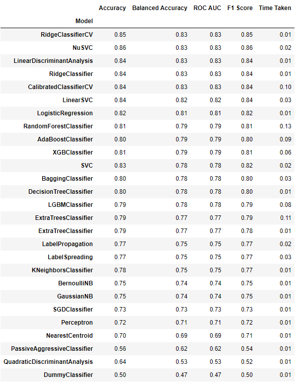
10. Evaluate Model

我们可以利用一些简单的 AutoML，将所有演算法/参数跑一遍并评估可行性：

from lazypredict.Supervised import LazyRegressor, LazyClassifier

cls = LazyClassifier(ignore_warnings=False, custom_metric=None)
models, predictions = cls.fit(X_train_std, X_test_std, y_train, y_test)

11. Save & Load Model

sklearn 有提供一内建存取方式

import joblib

model_file_name = 'model clf.joblib'
joblib.dump(clf, model_file_name)

读取方式：

clf_load = joblib.load('model clf.joblib')

接着试着输入资料来使用演算法
根据 EDA 的过程，会需要以下转换函式

import pandas as pd
import numpy as np

def convent_sex(sex):
    return 1 if sex=='male' else 0


def convnet_age(age):
    bins=[0, 12, 22, 30, 50, 60, 100]
    return pd.cut([age], bins, labels=[5, 2, 1, 4, 3, 0])[0]

dict1 = {'C': 0, 'Q':1, 'S':2}
def convnet_embarked(embarked):
    x = dict1[embarked]
    if x == 0:
        return 1, 0, 0
    elif  x == 1:
        return 0, 1, 0
    elif  x == 2:
        return 0, 0, 1

Method 1. 用 list 输入 (转成 np array/DataFram)

X = []
X.append([2, convent_sex('male'), convnet_age(31), 1, 2, np.log(32), *convnet_embarked('Q')])
X.append([1, convent_sex('female'), convnet_age(28), 1, 2, np.log(500), *convnet_embarked('Q')])
X=np.array(X)

丢进演算法中

X_test = stdsc.transform(X)
y = clf_load.predict(X_test)

y
>>  array([0, 1], dtype=int64)

Method 2. 用 dict 输入 (转成 np array/DataFram)

X_1 = {
    'pclass':2,
    'sex': convent_sex('male'),
    'age': convnet_age(31),
    'sibsp': 1,
    'parch': 2,
    'fare': np.log(32),
    'embarked_C': 1, 'embarked_Q': 0, 'embarked_S': 0
    }
X_2 = {
    'pclass':3,
    'sex': convent_sex('female'),
    'age': convnet_age(28),
    'sibsp': 1,
    'parch': 2,
    'fare': np.log(500),
    'embarked_C': 1, 'embarked_Q': 0, 'embarked_S': 0
    }

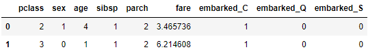
df = pd.DataFrame([X_1, X_2], index=[0, 1])
df

丢进演算法中

X_test = stdsc.transform(df)
y = clf_load.predict(X_test)

y
>>  array([0, 1], dtype=int64)

至此，就完成了经典题目：铁达尼号 的演算法演练了！

结论：

EDA 为在资料收集完成後的前处理，相对其他步骤来说，是最重要的步骤。
若资料处理（补偿、合并、删除）不够全面，将导致演算法 output 出一个不够全面的模型，使预测失准。
.
.
.
.
.
*补充1.：
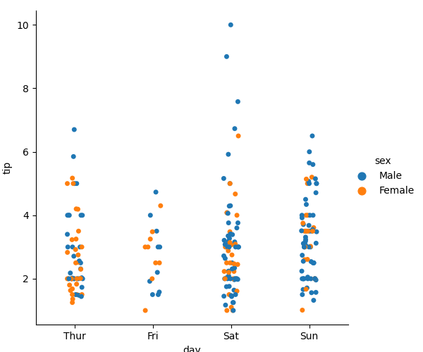
绝对散部图 sns.catplot：用在 x y 关系为绝对

sns.catplot(x='day', y='tip', data=tips, hue='sex')

.
.
.
.
.

Homework Ans：

使用假设检定，检定近40年(10届)美国总统的身高是否有差异?
(Data: president_height.csv)

1. Data Set

import pandas as pd
df = pd.read_csv('./president_heights.csv')
height = df['height(cm)']

2. 建立双样本：A. 近10届 (Sample2) B. 其他总统 (Sample1)

from scipy import stats
sample1 = height.head(len(df)-10)
sample2 = height.tail(10)

3. ttest 检定 (两样本独立)

z, p = stats.ttest_ind(sample1, sample2)
print(f'Z-value: {z}')
>>  Z-value: -2.69562113651512
print(f'P-value: {p}')
>>  P-value: 0.010226470347307223

4. 作图 (直方图)

# 根据 sample1 平均值 & 样本标准差，划出抽取 100000 次分配
s1_bar = np.random.normal(sample1.mean(), sample1.std(), 100000)
plt.hist(s1_bar, bins=100)
plt.axvline(s1_bar.mean(), c='y', linestyle='--', linewidth=2)

# 计算信心水准 95%，双尾检定结果(一边 2.5%)的 x_bar 值
ci = stats.norm.interval(0.95, s1_bar.mean(), s1_bar.std())
plt.axvline(ci[0], c='r', linestyle='--', linewidth=2)
plt.axvline(ci[1], c='r', linestyle='--', linewidth=2)

# 根据 mean + t*s 划出对立假设 x_bar 落点
plt.axvline(s1_bar.mean() + z*s1_bar.std(), c='m', linestyle='--', linewidth=2)
plt.savefig('pic HW9-2')
plt.show()

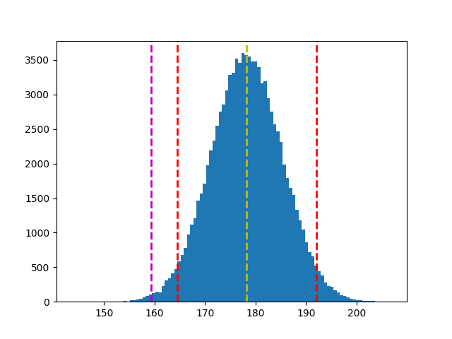
结论：近40年(10届)美国总统的身高有显着异於前任总统。
.
.
.
.
.

Homework：

请参考铁达尼号的流程，使用钻石清理资料来完成演算法。