前言

「指月录」卷二十八有道：

「见山是山，见水是水；见山不是山，见水不是水；见山仍是山，见水仍是水。」

这乃是学习深度学习时三种不同的境界，
从只看表面、看细节处再到综观全局，
就是「是山、非山、仍是山」的过程。

今天我们要使用预训练模型EfficientNet去提取图片特徵，
看看这些特徵就会体悟到刚刚的境界转换

载入套件

from tensorflow.keras.applications.efficientnet import EfficientNetB0
from scipy.spatial.distance import cdist
from sklearn.cluster import KMeans
from tensorflow.keras.utils import to_categorical
import tensorflow as tf
import pandas as pd
import numpy as np
import os
import matplotlib.pyplot as plt
import cv2

自定义函数

def prepare_data(data):

    image_array = np.zeros(shape=(len(data), 48, 48, 1))
    image_label = np.array(list(map(int, data['emotion'])))

    for i, row in enumerate(data.index):
        image = np.fromstring(data.loc[row, 'pixels'], dtype=int, sep=' ')
        image = np.reshape(image, (48, 48, 1))
        image_array[i] = image

    return image_array, image_label


def plot_one_emotion(data, img_arrays, img_labels, label=0):
    fig, axs = plt.subplots(1, 5, figsize=(25, 12))
    fig.subplots_adjust(hspace=.2, wspace=.2)
    axs = axs.ravel()
    for i in range(5):
        idx = data[data['emotion'] == label].index[i]
        axs[i].imshow(img_arrays[idx][:, :, 0], cmap='gray')
        axs[i].set_title(emotions[img_labels[idx]])
        axs[i].set_xticklabels([])
        axs[i].set_yticklabels([])


def plot_conv_feature(data, img_arrays, img_labels, label = 0):
    fig, axs = plt.subplots(4, 4, figsize=(16, 16))
    fig.subplots_adjust(hspace=.2, wspace=.2)
    axs = axs.flatten()
    for i in range(16):
        idx = data[data['cluster'] == label].index[i]
        axs[i].imshow(img_arrays[idx], cmap='gray')
        axs[i].set_title(f"feature {i}, cluster {label}", size = 20)
        axs[i].set_xticklabels([])
        axs[i].set_yticklabels([])


def convert_to_3_channels(img_arrays):
    sample_size, nrows, ncols, c = img_arrays.shape
    img_stack_arrays = np.zeros((sample_size, nrows, ncols, 3))
    for _ in range(sample_size):
        img_stack = np.stack(
            [img_arrays[_][:, :, 0], img_arrays[_][:, :, 0], img_arrays[_][:, :, 0]], axis=-1)
        img_stack_arrays[_] = img_stack/255
    return img_stack_arrays

读取资料

由於待会要下载的EfficientNet的输入层需要RGB彩色图片，
但我们只有灰阶图(单通道)，
所以用convert_to_3_channels将图片转成3通道，
注意！这里不是将图片变成彩色，只是单纯将第1通道复制贴到第2和第3通道。

df_raw = pd.read_csv("D:/mycodes/AIFER/data/fer2013.csv")
df_train = df_raw[df_raw['Usage'] == 'Training']
X_train, y_train = prepare_data(df_train)
X_train = convert_to_3_channels(X_train)  
y_train_oh = to_categorical(y_train)
emotions = {0: 'Angry', 1: 'Disgust', 2: 'Fear',
            3: 'Happy', 4: 'Sad', 5: 'Surprise', 6: 'Neutral'}

范例图片

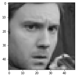
先选定一张我们要拿来萃取特徵的表情图片，
就决定是第一张了！

plt.imshow(X_train[0],cmap='gray')

读取EFN预训练模型

1. include_top: 是否需要原始模型的最上层(分类层)，因为我们不需要分类，所以选False。
2. weights: 选择哪种预训练权重，选择imagenet。
3. input_shape: 可以指定模型输入大小，预设是(224,224,3)。
4. pooling: 池化层方法选择，有avg和max可选，基本上都可以用。

efn = EfficientNetB0(include_top=False, weights='imagenet', 
                        input_shape=(48, 48, 3), pooling='max')

获得卷积层输出(低阶特徵)

在这里我们选择一个位於模型很前面的卷积层，获得低阶特徵(low-level)。
b1_result的shape为(1, 24, 24, 96)，
含意是1张图片透过卷积後，
原图缩小成(24,24)的特徵图，并且每张原图可对应到96个特徵图。

block1_conv_model = tf.keras.Model(efn.inputs, efn.get_layer(name='block2a_expand_conv').output)
b1_result = block1_conv_model(X_train[0]).numpy()
print(b1_result.shape)
# output: (1, 24, 24, 96)

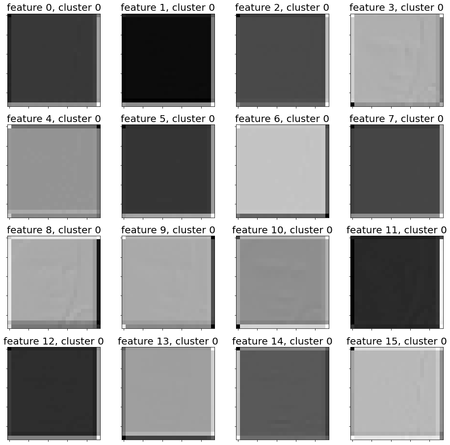
低阶特徵图范例

我们可以看出某些特徵图很有效地抓到了人脸的轮廓(例如: featrue 3, cluster 0)

获得卷积层输出(高阶特徵)

在这里我们选择模型最後一个卷积层，获得高阶特徵(high-level)。
top_result的shape为(1, 2, 2, 1280)，
含意是1张图片透过卷积後，
获得(2,2)的特徵图，并且每张原图可对应到1280个特徵图(feature map)。

top_conv_model = tf.keras.Model(efn.inputs, efn.get_layer(name='top_conv').output)
top_result = top_conv_model(X_train[0]).numpy()
print(top_result.shape)
# output: (1, 2, 2, 1280)

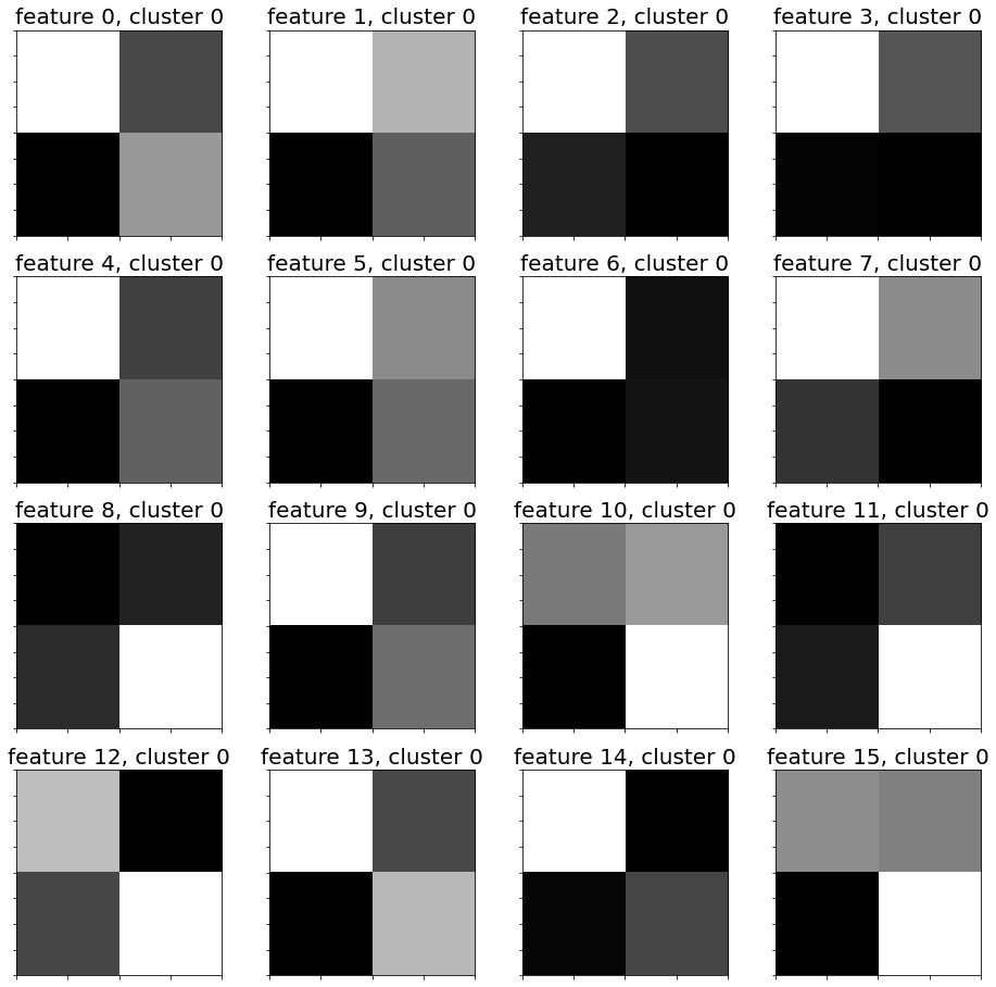
高阶特徵图范例

我们可以看出毕卡索再世，画出了原图的精神象徵(?) XD

笔记时间

1. 浅层网路解析度高，学到的是图片细节特徵(低阶)，像是边缘、棱角。
2. 深层网路解析度低，学到的是图片语义特徵(高阶)，是纵观全局的、抽象的。

结语

OK，今天学会了如何读取预训练模型，
并将自己的图片透过模型萃取出低阶与高阶的特徵。
这在业界是很常使用的技巧，
网路上也有许多大神提供的预训练模型。
明天就让我们来将这1280张高阶特徵图进行分群，
看看可以分成几群吧！